
Abstract
Understanding the implications of algorithmic trading calls for modeling financial markets at a level of fidelity that often precludes analytic solution. We describe how agent-based simulation modeling can be combined with game-theoretic reasoning to examine the effects of market variables on outcomes of interest. The approach is illustrated in a basic model where investors trade a single security through a continuous double auction mechanism. Our results demonstrate the feasibility of the approach, and raise questions about the use of spreads as a proxy for trading cost and welfare.
Program trading has been a reality for many years now, and the pervasiveness, speed, and autonomy of trading algorithms continue to reach new heights. Algorithmic strategies designed to respond to information within a few milliseconds or less are now widely deployed. The blink of a human eye, normally lasting over 0.3 seconds, may span hundreds of rounds of high-frequency trading (HFT). Although precise definitions or prevalence measurements of HFT are hard to come by, typical estimates agree that HFT accounts for over half of trading volume on U.S. equities and futures markets, and is increasingly common on currency exchange and fixed-income markets (Cardella et al. 2014).
With the ascent of algorithmic trading and HFT has come no small amount of public controversy, for example, about whether this practice contributed to the “flash crash” of May 6, 2010. Despite an abundance of available market data, understanding this episode is challenging because of the multiplicity of actors and complexity of interactions. This is reflected in necessarily complicated and nuanced characterizations of the role of HFT, as in the conclusion by Andrei A. Kirilenko et al. (2014) that HFT was not the proximate cause, yet HFT presence shaped the environmental conditions for the crash and accelerated price movements in response to the triggering event.
One way that prevalent algorithmic trading can shape the trading environment is through strategies that quickly withdraw liquidity when observations indicate a situation outside the normal operating conditions. This response is quite rational, given that underlying algorithms were derived and vetted on the basis of data from historical experience. When evidence presents that the current situation deviates qualitatively from historical conditions, the safe move is to turn off the algorithm. Of course, this is precisely the situation when the market is most in need of liquidity, so if such algorithms control the main liquidity sources this poses a clear stability risk.
Because the markets recovered minutes after they plunged, the May 2010 flash crash caused no general economic damage beyond harm to specific investors and traders caught in the wave—save perhaps the intangible erosion of confidence in the markets. The quick recovery is as mysterious as the precipitous drop, and there is no assurance that we will fare as well in the next flash-crash event. This next event is seemingly inevitable, as mechanisms in place to act as circuit breakers have limited ability to prevent or ameliorate them (Subrahmanyam 2013), and no other measures have qualitatively changed the general conditions of our financial markets. Subsequent smaller flash crashes in other financial assets (U.S. Treasury bonds in October 2014, U.S. dollars in March 2015) remind us that the prospect looms, and with it potential contagion across exchanges and asset classes, possibly triggering generalized panic impinging on the real economy.
The spotlight on HFT grew particularly intense in 2014 with the publication of Flash Boys, an engaging account by Michael Lewis (2014) of strategies employed by HFT firms to obtain and exploit speed advantages. Billions of dollars have been invested in new fiber-optic, microwave, and even laser-based communication networks, in the effort to shave milliseconds or microseconds off the information latency: the time it takes to transmit information across exchanges. To compete in this latency arms race firms spend additional billions on specialized hardware, co-location with exchanges, and development of streamlined software—possibly omitting error checks and other safety-enhancing features in the quest for ultimate speed.
Much of the debate about HFT revolves around the ramifications for real and perceived transparency and fairness of market operations; see, for example, criticisms by Haim Bodek (2013) about the proliferation of special order types catering to HFT strategies. This specific issue drew the attention of regulators at the U.S. Securities and Exchange Commission, who in January 2015 fined the exchange operator Direct Edge $14M for insufficient transparency about the availability and operation of special order types (Beeson 2015).
Some observers conclude that the state of U.S. equity trading markets is fundamentally broken (Arnuk and Saluzzi 2012) and call for sweeping reform. Others suggest that the apparent downsides of HFT are tolerable relative to the claimed beneficial effects of modern electronic trading. Some of the disconnects in this debate can be attributed to confounding qualitatively distinct forms of HFT, conflicting assumptions about market organization, or information hiding and obfuscation to protect proprietary interests.
Such issues can be addressed by careful research conducted in the public domain. Much of the finance literature on high-frequency trading (HFT) takes an empirical approach, and has come to mixed conclusions on the effects of HFT on overall market quality. For example, in a survey discussing the strategies, benefits, and costs of HFT, Charles M. Jones (2013) points to the positive role of HFT firms in market making and providing liquidity (Hendershott, Jones, and Menkveld 2011). The liquidity provided by algorithmic market makers, however, may be more erratic at high frequencies, and may be accompanied by increased adverse selection (Menkveld 2014). The effects of algorithmic trading operate along multiple pathways, with conflicting implications for market performance. As a result, most detached and deliberate commentators agree that uncertainty and concern about the ramifications of HFT, both potential and realized, are justified.
These uncertainties are difficult to resolve, in part because the factors at play in modern high-frequency trading are unprecedented. The most important new features in our view are the two following factors:
The very speed of operation renders details of internal market operations—especially the structure of communication channels and information—systematically relevant to market performance. In particular, the latencies (time lags) between market events (transactions, price updates, order submissions) and the point in time when various actors find out about these events become pivotal, and even the smallest differential latency can significantly affect trading outcomes.
The autonomy and adaptivity of algorithmic trading strategies takes them out of the scope of direct human control, and makes it challenging to understand how they will perform in unanticipated circumstances. The challenges are exacerbated by the increasing use of sophisticated machine learning techniques to derive trading strategies, and the fundamental multi-agent nature of the execution environment.
These two factors are closely interrelated, as autonomy is necessary for operation at superhuman speed. Some issues, such as interactions among adaptive and data-driven strategies, apply to algorithmic trading even when it is not conducted at high frequency (Easley, López de Prado, and O’Hara 2012).
In this article we outline a computational approach to analysis of financial markets that offers the fidelity needed to capture complex algorithmic trading environments yet is amenable to strategic reasoning based on game-theoretic principles. Following background on simulation modeling of financial markets, we present a simple yet realistic model environment and illustrate the approach for game-theoretic selection of trading strategies and reasoning about the effects of market conditions through equilibrium comparisons. Our results provide evidence for several propositions relevant to market performance and how it is assessed. Key findings include:
Modeling trader patience in terms of the time horizon they are willing to monitor and reenter markets, we find robustly that patient traders are able to achieve greater gains from trade, up to essentially full efficiency with sufficient horizon.
All else equal, more frequent market reentry and reduced fundamental volatility increase welfare.
The common use of quoted or effective spreads as a proxy for welfare is not a reliable guide for comparing market performance.
SIMULATION MODELING OF FINANCIAL MARKETS
Most of the finance community’s prior research on HFT takes an empirical approach, employing available order, quote, and transaction data streams to measure market activity and relate relevant variables. This has often yielded great insight and represents an essential form of inquiry. Analysis of available data is ultimately limited, however, with respect to counterfactual questions, such as the response of financial markets to rarely occurring shocks or the effects of alternative market rules and regulations. Answering such questions inherently requires models that incorporate causal premises, specifically, assumptions as to how trading behavior is shaped by environmental conditions.
Theoretical models can support such inference, and these also represent an important resource from the finance research literature. Trading in markets can be formulated as a game, and game-theoretic equilibrium concepts can be employed to characterize behavior in markets by rational agents. However, modeling algorithmic trading entails accommodating complex information and fine-grained dynamics, which often renders game-theoretic reasoning analytically intractable.
An alternative, computational, approach is to model financial markets in simulation. Simulation can faithfully capture complex market microstructure and trading interactions at arbitrarily fine degrees of temporal granularity. Algorithmic and other traders are cast as agents, with various objectives and information sources, and available actions as dictated by market rules. This approach, generally known as agent-based modeling (ABM), analyzes a complex social system through simulation of fine-grained interactions among the constituent decisionmakers (the agents), described and implemented as (usually simple) computer programs. ABM researchers in the social sciences typically justify adopting the agent-based approach on the basis of tractability, or avoiding restrictive assumptions about rationality or other characteristics (Tesfatsion 2006). Richard Bookstaber (2012) invokes these arguments and others in expressly advocating the development of agent-based models for investigating threats to financial stability.
ABM applications to financial trading date back to the 1990s, notable early models including those by Moshe Levy, Haim Levy, and Sorin Solomon (1994) and the Santa Fe Artificial Stock Market (Arthur et al. 1997). Agent-based financial models facilitate consideration of heterogeneous agent types (Boswijk et al. 2007), and multiple forms of learning (LeBaron 2011). Researchers have employed ABMs to shed light on central issues in today’s financial markets, such as the impact of a transaction tax (Fricke and Lux 2015), and conditions that can produce instabilities reminiscent of the 2010 flash crash (Lee, Cheng, and Koh 2011; Paddrik et al. 2012).
In our own previous work we have used agent-based simulation of financial markets to model a variety of trading scenarios. We focus on the impact of algorithmic trading on allocative efficiency (social welfare), which is a measure of how well markets distribute resources (in this context, financial securities) to market participants. Greater efficiency means improvements (in aggregate) in investors’ gains from trading.
In one study, we investigated the effect of latency arbitrage, an HFT strategy that exploits speed advantages in identifying price disparities across fragmented markets (Wah and Wellman 2013). We found that latency arbitrage harms market efficiency, not even counting the costs of the latency arms race. We proposed that this arms race can be eliminated by replacing continuous-time trading with frequent-call markets, a mechanism whereby orders accumulate and are matched periodically, for example, once per second. Frequent-call markets neutralize tiny speed advantages (Budish, Cramton, and Shim 2015) and can improve market efficiency in many circumstances.
One of our recent studies examines the welfare effects of market making, finding that market makers generally improve efficiency, but provide benefits to investors only when the investors are sufficiently impatient (Wah and Wellman 2015). The model we present here follows the configuration of this study and reports an extended analysis of trading strategies (without the market makers) explored there.
SECURITY TRADING MODEL
Our analysis focuses on a single security traded in a two-sided market. Though the model is simple, it captures key characteristics of real-world market mechanisms and trading behavior. Here we present a basic description of market operation, and the objectives and strategies of traders. The appendix provides a more detailed mathematical description.
The market operates over a finite time horizon, which we call T. Agents enter and reenter the market at random intervals to trade. On each arrival these traders submit a limit order to the market (replacing their previous order, if any), indicating the price at which they are willing to buy or sell a single unit of the security.
The market mechanism is a continuous double auction (CDA) (Friedman 1993), which means that a new buy or sell order transacts immediately whenever it matches an existing order in the market. The trade executes at the price of the incumbent order. If an order does not match, it is added to the CDA’s order book. The CDA maintains price quotes reflecting the best outstanding orders. These quotes comprise two parts: a bid quote BID reflects the highest current buy offer, and ask quote ASK the lowest current offer to sell.
The market environment is populated by a set of traders, representing investors. Each investor has an individual valuation for the security made up of private and common components. The common component is represented by a fundamental value, which can be viewed as the intrinsic value of the security. This fundamental value varies over time according to a stochastic process.
The private component of value is a specific agent’s reason for trading. For example, an agent may have positive value for a security that complements its portfolio (for example, it hedges other risk), and negative value for undiversified risk. Similarly, the need for savings or liquidity is reflected in the private value.
The common and private components are effectively added together to determine the agent’s valuation of the security. Agents accrue private value on each transaction, and at the end of the trading horizon evaluate their accumulated inventory on the basis of the end-time fundamental.
Given a market mechanism and valuation model, investors pursue their trading objectives by executing a trading strategy in that environment. As noted, we assume that traders arrive stochastically at the market over a time horizon, and at each arrival have the opportunity to submit a limit order to buy or sell a single unit of the security. The strategy defines how this order is generated, on the basis of price quotes and current holdings.
Though the CDA market mechanism and environment as described here are relatively simple, the associated bidding game is quite complex, owing to the incompleteness of information (private valuations) and the dynamics of arrivals and repeated trading. No analytic solution—nor any constructive theoretical characterization—is known for this or similar CDA games, and so the literature has generally relied on simulation studies. Many previous works have explored CDA bidding strategies (Das et al. 2001; Friedman 1993; Wellman 2011), so there is a body of ideas to work with. Many of the proposed solutions are variations of the so-called zero intelligence (ZI) family of bidding strategies (Gode and Sunder 1993), and that is the class of approaches we consider here.
In the ZI bidding strategy, agents determine an amount of surplus to ask for, and submit a corresponding limit order. The strategy parameters Rmin and Rmax (0 ≤ Rmin ≤ Rmax) govern the range of surplus requests. Our extended version of ZI employs a third parameter, η ∊ [0,1], which is a threshold determining whether to just take the currently available surplus based on the price quotes. The details of our strategy implementation are provided in the appendix.
Although ZI is quite simplistic as a trading strategy, it does reflect cognizance of common and private value components, and through setting of the strategic parameters (Rmin, Rmax, η) it accommodates a spectrum of surplus-demanding behavior. The most effective settings of these parameters vary depending on the environment (such as number of other traders, valuation distributions, time horizon, arrival rate) and the strategies employed by other traders. Any conclusions for market performance, therefore, are sensitive to choice of these ZI parameters. We have developed a game-theoretic process for choosing strategic parameters in simulation models, described in detail in the next section.
EMPIRICAL GAME-THEORETIC ANALYSIS
A financial market simulation model provides a way for an experimenter to directly answer questions of the form “What happens when the trading strategies <fill in strategy set> interact in environment <fill in environment specification>?” Choice of environment specification is driven by the target subject of study, and may be informed by existing models and data. The choice of strategies, however, is up to the market participants, and since strategies are not generally observable in market data, the experimenter must consider how traders would be likely to act in a given market situation. The conventional economic assumption is that traders rationally pursue their objectives, and the standard economic approach to strategy choice relies on reasoning based on rationality criteria.

Empirical Game-Theoretic Analysis
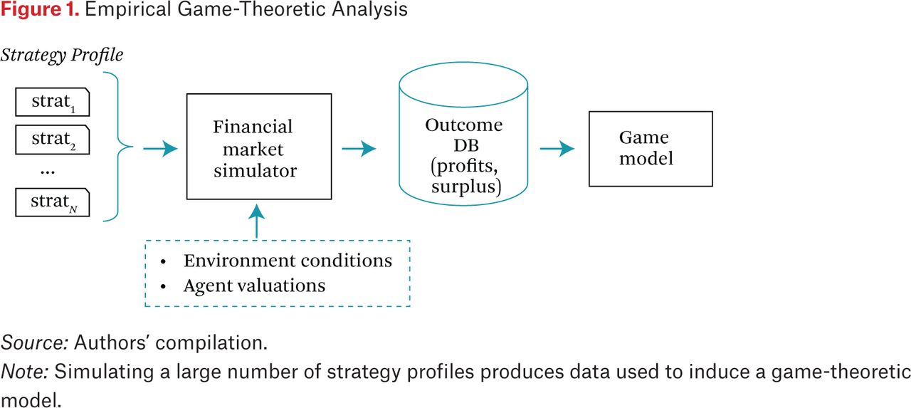
The empirical game-theoretic analysis (EGTA) approach incorporates such reasoning in a simulation-based framework. Figure 1 illustrates how EGTA generates a game model from financial-market simulations. First, we configure the financial-market simulator on the basis of the market mechanisms (number of markets, continuous versus periodic clearing, quoting policies), environmental conditions (numbers and types of traders, communication latencies), and agent valuations (fundamental process and private component distributions) we wish to study. These configurations may have both structural and parametric elements. For example, we used this simulator to investigate latency arbitrage, an HFT tactic that exploits speed advantage to profit in fragmented markets. Our study of latency arbitrage (Wah and Wellman, 2013) was based on a two-market model, with individual-market and global public price quotes (the national best bid and offer, or NBBO) available to regular and high-frequency traders at differential latency. Given this structure, we then varied the latency parameter to evaluate its effect on market outcomes. That study also compared to single-market models, employing CDA or call-market clearing mechanisms.
The simulator configuration includes a specification of the numbers of players in various roles. Each role is associated with a set of available strategies. Within each role, players are treated as ex ante symmetric. (This is without loss of generality, as we can always associate a unique role with each player.) In our study of market making, for example, there were two roles: background investor and market maker. In the current study, we consider only the investor role. The strategy set is the family of ZI bidders defined earlier.
Once configured, we can feed into the market simulator a strategy profile, defined as an assignment of strategies to each player. In our case, assigning a strategy means assigning the ZI parameters (Rmin, Rmax, η) for each trader. Each simulation run produces an outcome (set of trades), which in turn defines a net surplus for each trader (value of final holdings minus cash flow). This can be interpreted as the agent’s payoff for that run of the market game. In general, given the stochastic nature of the market simulation (random draws of valuations, fundamental time series, agent arrival patterns), we require many runs to yield accurate estimates of payoffs for any given strategy profile.
To perform EGTA of a particular scenario, we evaluate a large number of strategy profiles in this manner, collecting the estimated payoffs in an outcome database. From this data we then induce a game model. This game model may generalize to nonsimulated profiles through regression (Vorobeychik, Wellman, and Singh 2007); however, in many cases (such as this study) we generate an incomplete game model that includes payoff estimates only for simulated profiles.
Given a game model, we can perform any of the usual game-theoretic analysis operations, for example, computing Nash equilibrium (NE). In our study, we focus on identifying symmetric mixed-strategy NE. Given a set of evaluated profiles, our algorithm starts by finding the maximal complete subgames (henceforth referred to as subgames): sets of strategies such that all profiles are evaluated. For each subgame, we compute subgame equilibria by the replicator dynamics algorithm (Gintis 2000), which starts from a particular probability distribution over strategies, then increases the probability of those strategies that perform better than average. We run this replicator dynamics method initialized at a diverse set of points in the simplex, then test whether these subgame equilibria are equilibria in the full game by evaluating all deviations outside the subgame.
In principle, the EGTA approach could apply to a game of any size. In practice, we are limited by the computation available for simulation, which is proportional to the number of profiles evaluated. Financial markets often involve a large number of traders, and there is a large space of possible strategies. Even if we restrict attention to ZI strategies, there is a three-dimensional parametric space of strategy settings. Let N denote the number of traders, and S the number of strategies. In this study, we investigate markets with N = 25 and N = 66, and consider S = 9 distinct settings for the ZI strategy. A symmetric game has

distinct strategy profiles (that is, the number of different ways of drawing N items from N – S + 1 candidates), and so even games of this modest size cannot be explored exhaustively. For example, with N = 25 and S = 9, the number of profiles is 13.9 million.
To enable analysis of games at this scale, we employ an approximation technique called deviation-preserving reduction (DPR) (Wiedenbeck and Wellman 2012). DPR approximates an N-player game by a smaller k-player game with the same strategy set. The method estimates payoffs in the reduced game based on a mapping from select profiles in the full game. For example, with N = 25 and k = 5, the payoff to the player playing strategy a in the reduced-game profile (a, b, c, d, d) would be obtained by simulating a 25-player profile where one agent plays a and the other 24 are divided across the remaining strategies as follows: 6 each play b and c, and 12 play d. This reduction is termed “deviation-preserving” because it accurately reflects the first player’s relative payoffs for playing alternative strategies in this context. It is still an approximation, however, because the other players are treated as aggregates. This technique has been shown to produce good approximations for purposes of equilibrium identification in a variety of large games. In this study, we employ 5-player reductions for the N = 25 cases, and 6-player reductions for N = 66.
EXPERIMENTAL SETUP
The experiments reported here elaborate the analysis of trading environments investigated in our prior work (Wah and Wellman 2015), focusing on the games with no market maker present. Traders follow the ZI strategy described, with settings (Rmin, Rmax, η) selected from the following set of thirteen triples:
{ (0,65,0.8), (0,125,0.8), (0,125,1), (0,250,0.8), (0,250,1), (0,500,1), (250,500,1), (0,1000,0.8), (0,1000,1), (500,1000,0.4), (0,1500,0.6), (1000,2000,0.4), (0,2500,1) }
This set was determined in a fairly ad hoc manner. We seeded it with all of the η = 1 strategies above, then extended it to include some η = 1 cases based on finding improvements from initial equilibrium candidates. We also tried some strategies with Rmin ∊ {2500,5000} and Rmax ∊ {10000,15000}, but these never appeared in equilibrium so were discarded.
We consider three instances of the market environment, labeled A, B, and C. All three assign traders a private valuation generated with variance parameter  and qmax = 10. (See the appendix for definitions of these and other parameters.) The global fundamental has a mean value
  and evolves with mean reversion κ = 0.05. The environment differences are focused on two parameters:
Agent reentry rate: λ = 0.0005 (environment A) or λ = 0.005 (environments B and C)
Fundamental shock variance:
 (environments A and B) or (environment C)


For each environment, we consider three different time horizons T (in 1,000s) and two settings for number of traders N. For N = 25 we considered an additional horizon T = 24. Thus we explored a total of 21 games using the EGTA approach. We label each game according to the environment (A, B, C) and time horizon T, where T ∊ {1, 4, 12, 24}; for example, B12 is environment B with time horizon 12.
RESULTS
To analyze a particular game configuration we perform a systematic search, evaluating strategy profiles through simulation with the goal of identifying equilibria. Our search process starts by considering each ZI strategy in self-play—the nine pure symmetric profiles where every agent plays the given strategy. We then iteratively generate additional profiles to simulate according to the following criteria:
For any subgame equilibrium that is not refuted in the full game, evaluate all deviations outside the subgame.
Extend a refuted subgame equilibrium by adding the best response strategy to the set of strategies in that equilibrium profile’s support.
Note that deviations and subgame profiles are selected on the basis of the reduced 5- or 6-player games defined by our DPR approximation. The payoffs for these reduced games are estimated based on simulation results from corresponding full-game profiles.
For each of the 21 games analyzed, this process succeeded in identifying at least one and up to three distinct symmetric equilibria. This typically required evaluating 1,000 or 2,000 full-game profiles, with an actual range of 553 to 4,167. Each profile evaluated was simulated at least 20,000 times. Overall, the computation deployed for this study occupied dozens of cores on a large-scale computing cluster for much of the time over a period of several months.
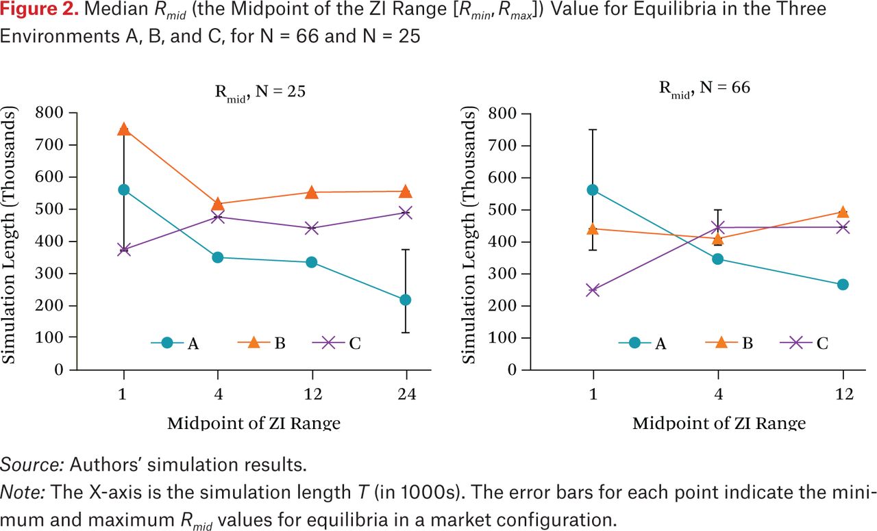
A summary of the equilibria across environments is presented in figure 2. For each market size (25, 66) and each environment (A, B, C) we plot a series of points corresponding to the five time horizons T considered. Each point summarizes the equilibrium ZI parameters using the average of surplus-request midpoints, Rmid = (Rmin + Rmax)/2, with the average weighted by probability in the equilibrium profile. For games with multiple equilibria, we display the range of Rmid values using error bars.
The Rmid statistic for a profile represents the average surplus requested in a trader limit order, but only approximately, as it ignores the effect of the quote threshold parameter η. Figure 2 suggests some general trends in this statistic, but we are reluctant to draw strong conclusions, given the roughness of this measure and the inconsistency in the observed trends. Nevertheless, we do generally see that the thinner markets (N = 25) have higher surplus requests, and that there is some tendency for these requests to decrease with time horizon, particularly for environment A.

Median Rmid (the Midpoint of the ZI Range [Rmin, Rmax]) Value for Equilibria in the Three Environments A, B, and C, for N = 66 and N = 25
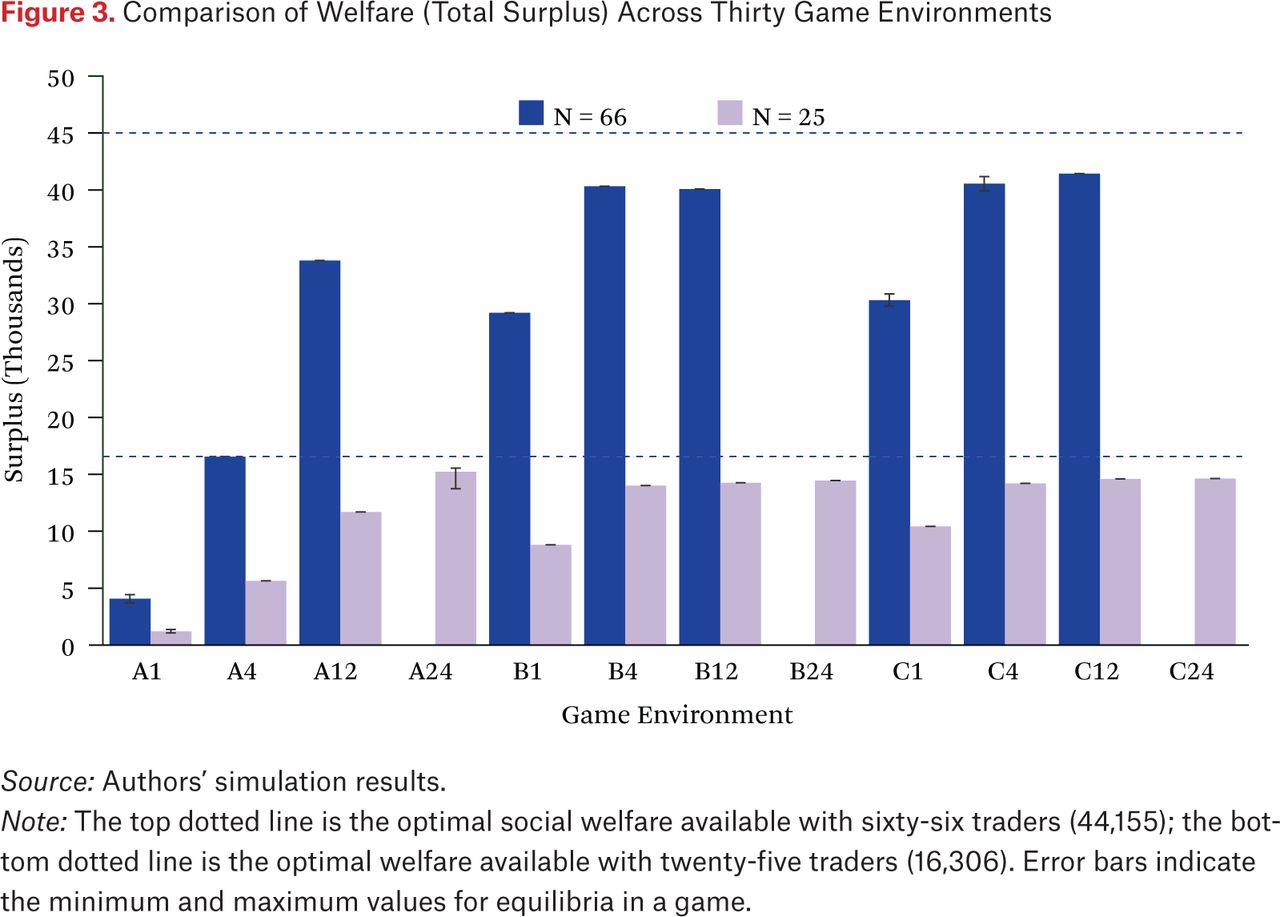
Perhaps the most salient outcome variable is market efficiency, which we measure by total surplus. For each equilibrium we evaluated total surplus from 10,000 sample runs over the full-game mixed profile. Figure 3 displays the market efficiency exhibited in equilibrium across our 21 games. For this variable, the relationships are quite apparent. Welfare generally increases with time horizon. The reason is that with longer horizons, traders have more reentries and thus greater opportunity to find mutually beneficial trades. With enough time, the ZI traders are able to achieve a high fraction of full efficiency in equilibrium.

Comparison of Welfare (Total Surplus) Across Thirty Game Environments
It is also apparent from figure 3 that environments with more frequent trader entries (B and C compared to A) have higher surplus, for any given horizon. This holds for the same reason that extending horizon improves efficiency. Closer inspection of the figure reveals that when holding arrival rate and horizon fixed, for N = 66, reducing fundamental volatility (moving from environment B to C) increases efficiency to a small but consistent degree. It seems that with thick markets, high variance on the fundamental often leads to extramarginal trades, which then require additional entries to correct.
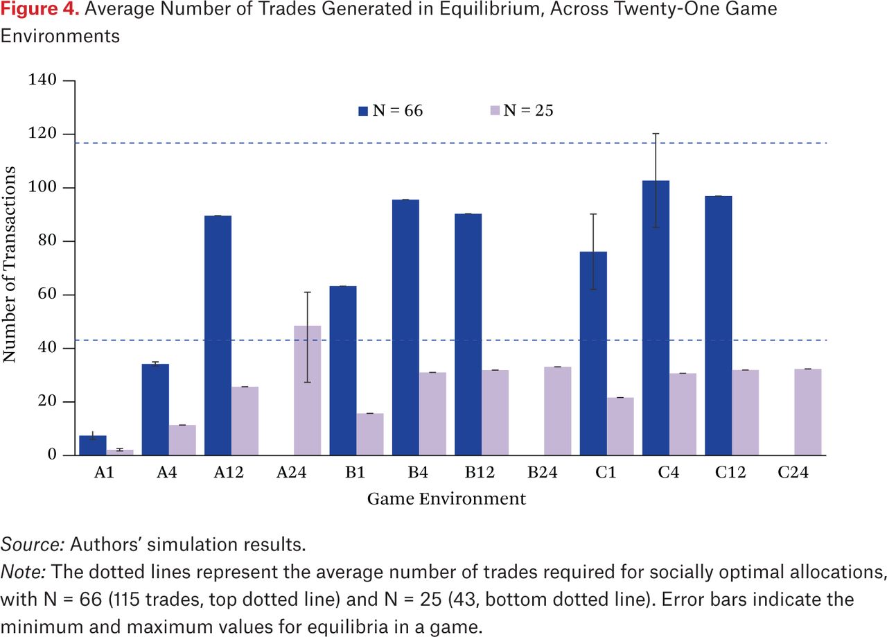
Inspection of the number of trades produced in equilibrium (figure 4) is also illuminating. A few equilibrium instances generate high efficiency but produce more trades than optimal, indicating that these runs involve agents who make trades and reverse them on subsequent entries.

Average Number of Trades Generated in Equilibrium, Across Twenty-One Game Environments
SPREADS AND MARKET EFFICIENCY
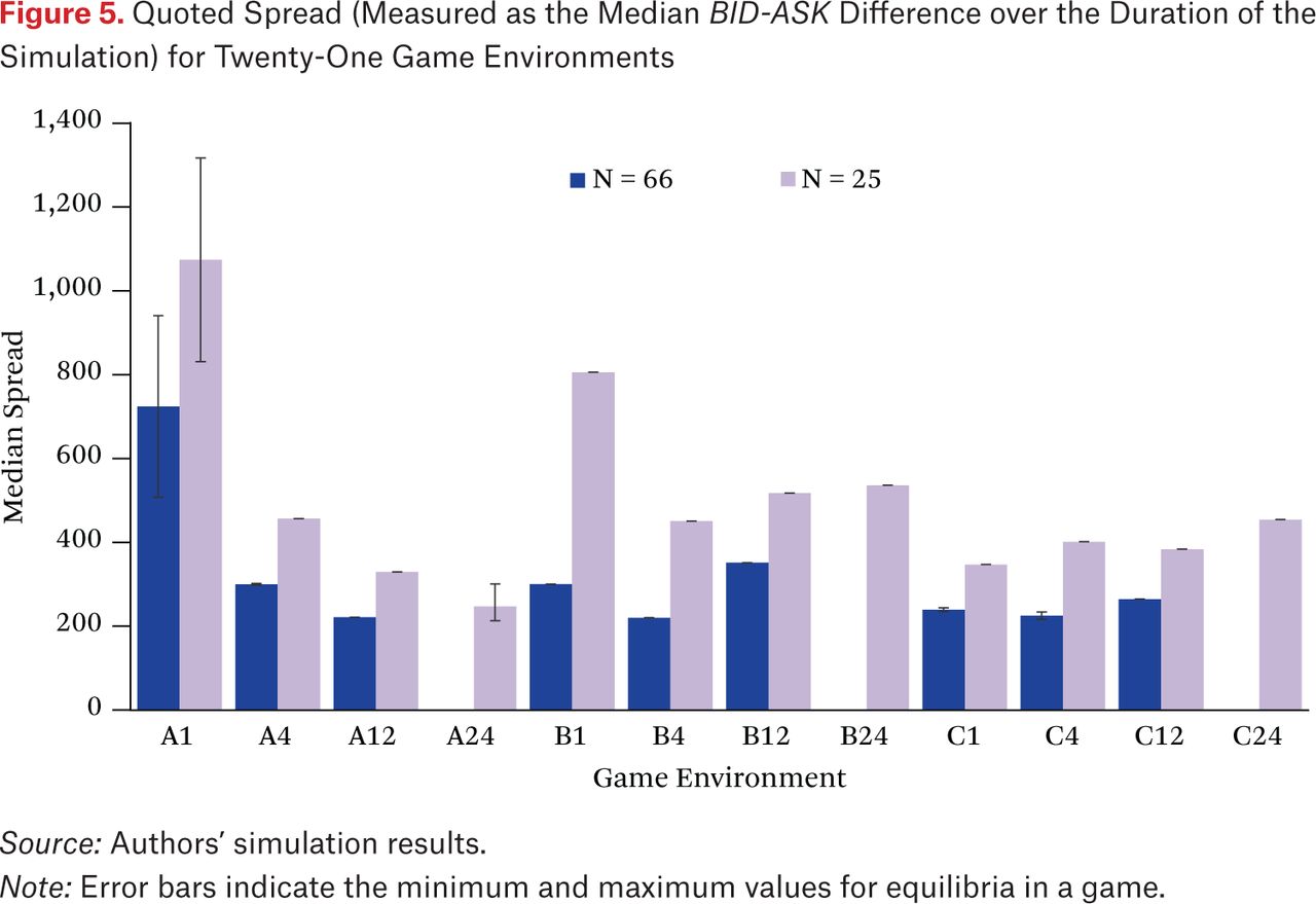
The final question we examine with data from our EGTA study concerns the reliability of spreads as a proxy for market efficiency or welfare. True transaction cost, or the difference between the price of execution and the true value of the security, is a measure of the net change in welfare of market participants. When welfare is not directly observable, as is generally the case for real-world data, proxy measures for transaction costs can be employed to estimate changes in welfare (Goettler et al. 2005). Estimation of the cost of trading relies on the intuition that in the absence of execution costs, transactions would occur at the underlying value of the security. As such, the difference between trade price and any proxy for the value of the security gives an estimate of the cost of execution (Bessembinder and Venkataraman 2010). There are multiple ways to estimate these execution costs. The simplest of these is the quoted spread, which is defined at a particular time point as the difference between the BID and ASK quotes. We summarize quoted spread for a scenario run as the median spread over all time points. Figure 5 presents statistics on quoted spreads for equilibrium trading in our 21 game configurations. As one would expect, spreads are always greater in thinner markets, all else equal. We also tend to find smaller spreads in the scenarios exhibiting greatest surplus (compare figure 3), although this correspondence is rough and inconsistent at best.

Quoted Spread (Measured as the Median BID-ASK Difference over the Duration of the Simulation) for Twenty-One Game Environments
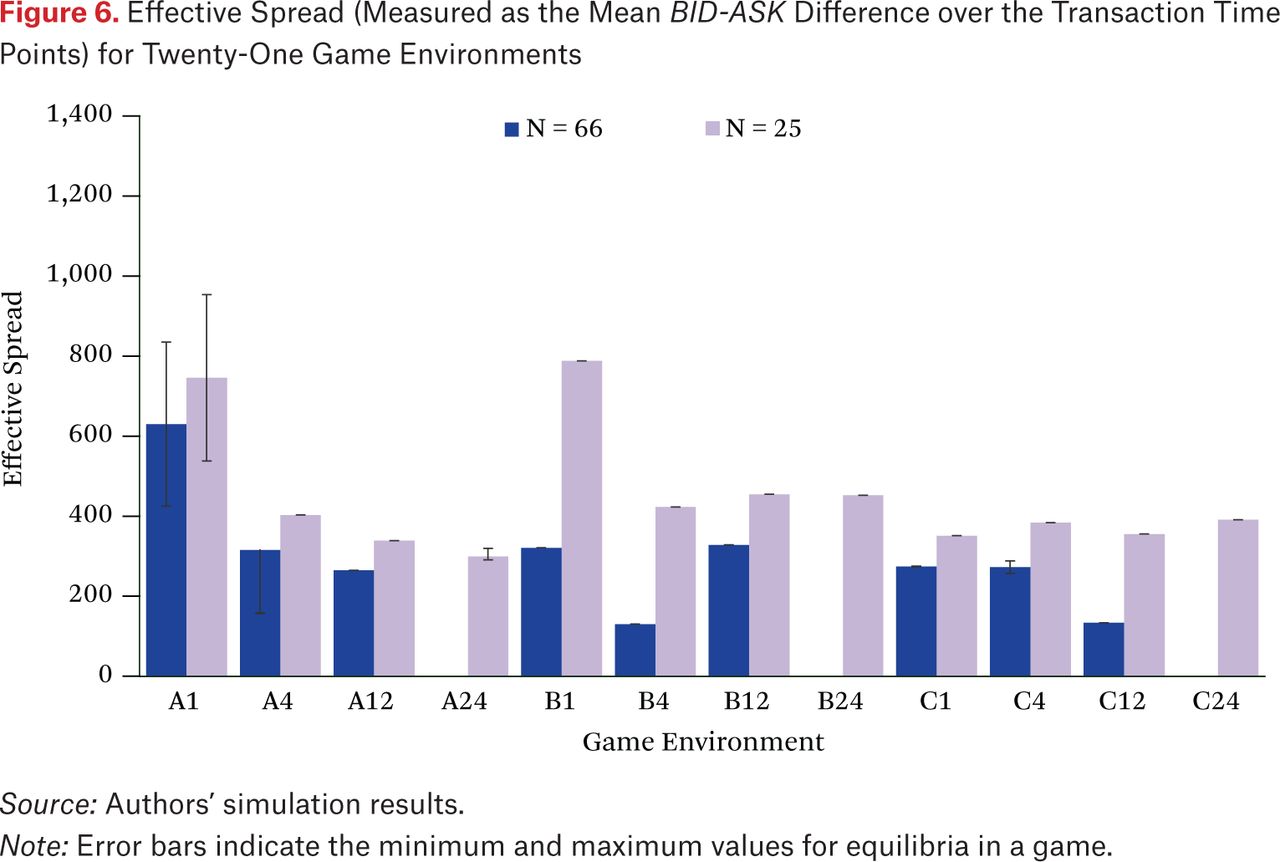
If quotes vary significantly over time, aggregating quoted spreads over all time points may not accurately reflect trading costs. An alternative is the effective spread, which focuses on spreads in effect at the time of actual trades (Bessembinder 2003; Madhavan et al. 2002).1 Specifically, our aggregate measure of effective spread takes the mean BID-ASK difference over all times when a trade occurs. These effective spread values for the equilibria found in each environment are shown in figure 6.

Effective Spread (Measured as the Mean BID-ASK Difference over the Transaction Time Points) for Twenty-One Game Environments
We see that effective spreads are sometimes substantially lower than the quoted spreads and never vice versa (figure 5), reflecting the fact that a new limit order is more likely to match at times when the spread is tight. Nevertheless, quoted and effective spreads are highly correlated, suggesting that quoted spreads can serve as a predictor for effective spreads. As for quoted spreads, tighter effective spreads often correspond to increased welfare in the corresponding environment, but this is not consistently the case.
Such inconsistency may not be surprising, given that other factors also vary systematically across game instances. We tested the correspondence of spreads and welfare within games by examining cases of multiple equilibria. Six of our games have multiple equilibria, and in only two (that is, one-third) does the ordering of quoted spread accord with the ordering of welfare. For effective spread, the correspondence also holds in only two of six cases.
To further examine the efficacy of spread measures as a proxy for welfare, we simulate 10,000 samples of five pure-strategy profiles for N = 66 and N = 25 under fixed market configuration (game B12). The strategies of these profiles all belong to the ZI family, with the following ranges (η = 1 unless otherwise stated):
B12a: ZI[0, 125] with η = 0.8
B12b: ZI[0, 250]
B12c: ZI[0, 1000]
B12d: ZI[0, 2500].
B12e: ZI[500, 1000] with η = 0.4
In each of these profiles, all N traders play the specified strategy. The surplus of each profile is shown in figure 7, and the corresponding spread measures are in figure 8. We measure quoted spread as a time series across the duration of the simulation and report the median spread, and we report effective spread as the mean over all transactions.
We find that for both populations, the surplus is the lowest for profile B12e and is relatively constant for profiles B12a to B12c. Both spread measures, in contrast, widen over the a-to-e range, which properly reflect the increase in welfare from c to e, but fail to accurately mirror the flat welfare rankings in profiles B12a to B12c. This is particularly true for quoted spread. Effective spread comes closer to matching the flat area overall surplus for N = 66, but its correspondence breaks down in the thinner market with 25 traders, for example in the increased spread from B12b to B12c.
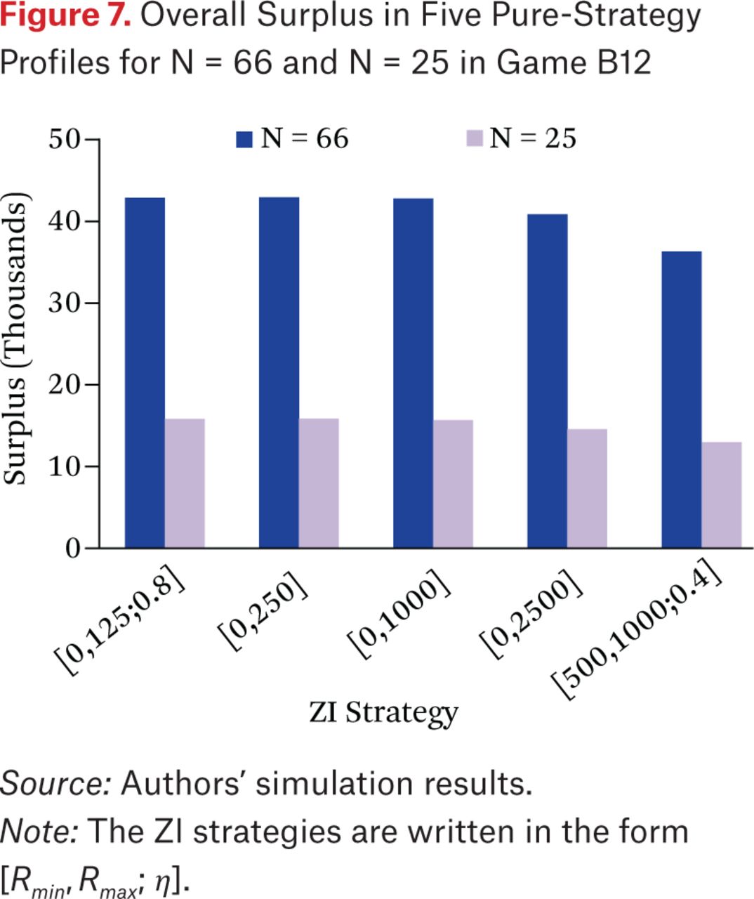
Overall Surplus in Five Pure-Strategy Profiles for N = 66 and N = 25 in Game B12
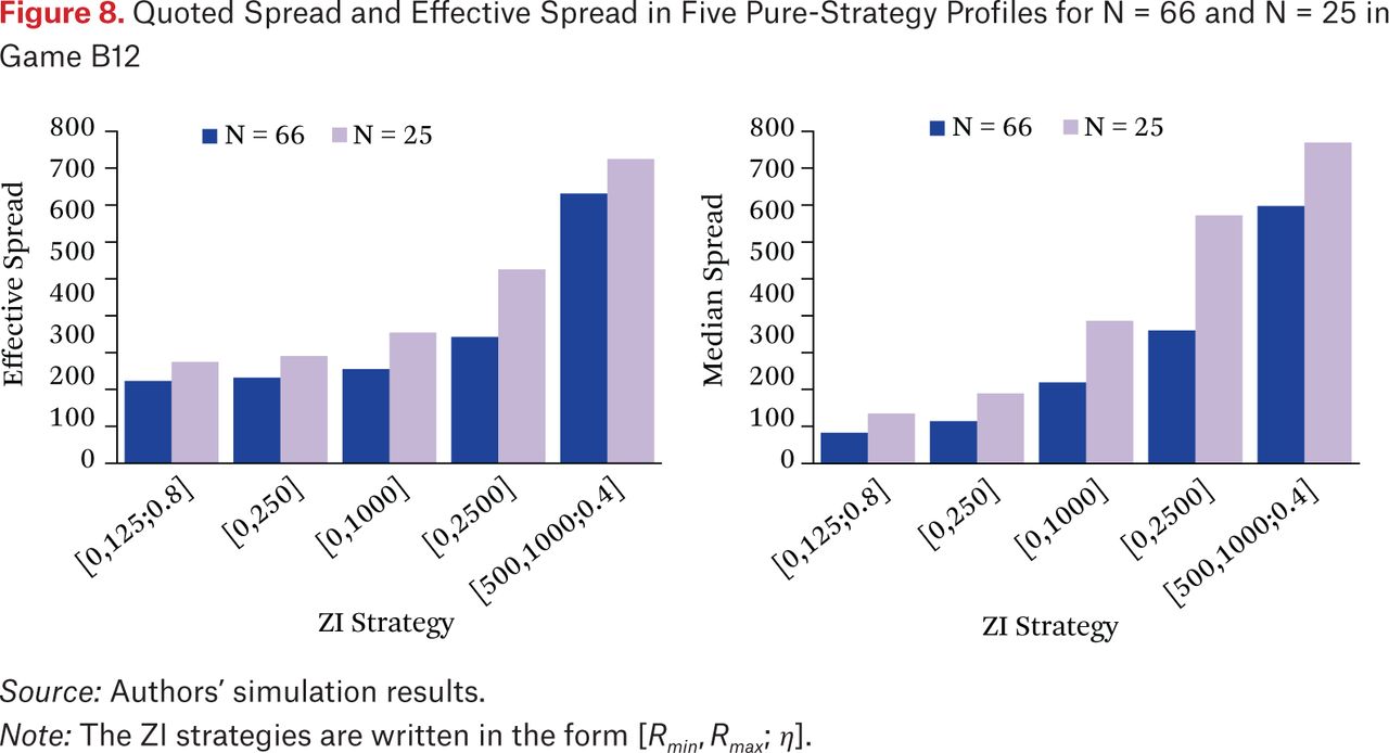
Quoted Spread and Effective Spread in Five Pure-Strategy Profiles for N = 66 and N = 25 in Game B12
As true value of the security is unobservable in real data, proxies such as quoted and effective spread may often be the best available predictors of transaction costs. However, accurately computing effective spreads from real data is often difficult, as it is not always readily apparent from historical trade prices and quotes which price quote corresponds to a given transaction, especially when order-level data are not available. In addition, effective spread measures can be particularly sensitive in electronic markets, with frequent quote updates and more active trading (Piwowar and Wei 2006).
A more fundamental problem with effective spread, however, is that it was developed for intermediated markets, where prices are set by a middleman, such as a dealer. In a pure limit-order market, prices are determined by arriving traders and thus are not necessarily equal to the expected value of the security. Ronald L. Goettler, Christine A. Parlour, and Uday Rajan (2005) demonstrate that the midpoint of the BID-ASK spread is not a good proxy for a security’s true underlying value. Given that it emphasizes the surplus of the trade-initiating order submitter and omits the surplus of the incumbent order submitter, effective spread is not a generally representative estimate of welfare.
CONCLUSIONS
We have presented an approach to strategic reasoning, using agent-based simulation models, for application to understanding trading behavior in financial markets. Contrary to views often expressed by advocates (and respectively, critics) of agent-based modeling and game-theoretic analysis, the two methods are actually quite complementary, together supporting principled strategic analysis of complex dynamic scenarios. We illustrated the approach by deriving and analyzing equilibrium trading strategies for a variety of continuous double auction scenarios, differing in number of traders, trading horizon, arrival rate, and fundamental volatility.
Our study confirms several expected relationships among market outcomes, and particularly underscores the importance of trader reentry in achieving efficient outcomes in continuous double auctions. Data from simulations were also instrumental in demonstrating the limitations of relying on proxies such as price quotes for statistics of central interest, such as welfare.
The unobservability of key elements (strategies, welfare) in empirical data provides a strong impetus behind the simulation approach to modeling financial markets. Our simulation studies of latency arbitrage and market making have shed light on the costs and benefits of such strategies, in terms of their effects on the welfare of investors. These works highlight the importance of distinguishing among different roles of algorithmic trading, separating the deleterious practices (latency arbitrage) from those that improve market performance (liquidity provision to impatient investors). This argues against broad-brush regulatory policies that raise the costs of algorithmic trading across the board, in favor of more targeted interventions that deter the harmful forms of algorithmic trading without unduly burdening beneficial practices.
Our ongoing research is applying the approach illustrated here to further key questions in the behavior of financial markets, for example: comparing continuous and periodic trading rules, effects of competition among market makers, and adoption of alternative market mechanisms (Wah, Hurd, and Wellman 2015). Models combining rich simulation with game-theoretic reasoning can play a constructive role in evaluating alternative market mechanisms and enhancing our understanding of the effects of algorithmic trading in a wide range of scenarios.
APPENDIX
Mathematical Model Formulation
In the Appendix we provide further technical details of our models of the market environment and agent trading strategies.
Market Operation and Agent Valuations
We model a single security traded in a two-sided market. Prices are integers, which means they are discretized at a tick size of any desired granularity. Time is also defined on a discrete domain, with finite horizon T. Agents arrive to submit their limit orders according to a Poisson distribution, with a rate parameter λ defining the probability of arriving in each unit time. The market mechanism is a standard limit-order market, or continuous double auction (CDA).
Traders value the security on the basis of a common fundamental value, in combination with an individual-specific private value. We denote by rt the fundamental value for the security at time t. The fundamental time series is generated by a mean-reverting stochastic process:

Parameter κ ∊[1,0] specifies the degree to which the fundamental reverts back to the mean  , and parameter
  is a random shock at time t.
The private valuation component for agent i is a vector

where qmax > 0 is the maximum number of units an agent can hold (either long or short). Θt specifies the marginal private benefits to agent i of trading single units, according to i’s current net position. Element θiq is the incremental private benefit obtained from selling one unit of the security, given current position q, where positive (negative) q indicates a long (short) position. Similarly,  is the marginal private gain from buying an additional unit given current net position q. This representation is similar to the model of Goettler, Christine A. Parlour, and Uday Rajan (2009).
Agent i’s private valuation vector is generated by drawing 2 qmax values independently from a Gaussian distribution,  . To ensure that the valuation reflects diminishing marginal utility, that is, θqʹ ≥ θq for all qʹ ≤ q, we sort the drawn values before assigning the vector Θi.
At the end of the trading horizon, an agent’s total value is the sum of private values accrued on each transaction, plus the worth of its final holdings evaluated at rT, the end-time fundamental value. Agent i’s valuation vi(t) for the security at time t therefore depends on its current position qt and the value of the common fundamental at the end of the trading horizon:
The surplus of a trade is the difference between valuation (including both common and private components) and transaction price. For a single-quantity limit order transacting at time t and price p, a buyer B obtains surplus vB(t) – p, whereas seller S obtains surplus p – vS(t). Since the price and fundamental terms cancel out in exchange, the total surplus achieved when B buys from S is  , where q(i) denotes the pre-trade position of agent i.
Trading Strategies
An agent’s trading strategy governs how it generates a limit order each time it arrives to the market, as a function of its state and information. To simplify the strategy structure, we assume that the trader flips a coin on each arrival to decide whether its order on that round will be to buy or to sell. As a result, agent i’s decision boils down a price for its new limit order, as a function of its valuation vector Θi, current holdings q(i), and its history of market observations (transactions and price quotes).
In the zero intelligence bidding strategy, agents bid for a randomly determined amount of surplus. Our extended version of ZI employs three parameters: Rmin and Rmax (0 ≤ Rmin ≤ Rmax) define the range of surplus requests, and η ∊[1,0] is a threshold for taking the currently available surplus. Specifically, a ZI trader i constructs its bid as follows:
Assess its valuation vi(t) at the time of market entry t, using an estimate r̂t of the end-time fundamental rT. The estimate is simply an adjustment of the current fundamental rt, accounting for mean reversion:
Determine its requested surplus s, by drawing uniformly from the interval [Rmin, Rmax].
If the surplus available at the current price quote is at least ηs, then submit an offer at the quoted price. Otherwise submit a limit order requesting surplus s. For instance, if the agent is buying, its bid price is given by:

Note that a trader with η = 0 accepts any profitable quote, and one with η = 1 bids the same, regardless of the current quote.
For example, consider a trader with valuation v applying a ZI strategy with parameters Rmin = 0, Rmax = 1000, and η = 0.6. On entering the market, it first flips a coin to decide whether to buy or sell. Supposing the coin flip dictates BUY, it then draws a random surplus request s ~ U[0,1000], which for example yields s = 700. It therefore aims to buy at a price 700 below its valuation. If it can buy right now at a price of 700η = 420 less than v (that is, if ASK ≤ v – 420), however, it submits a price at the current market value. Otherwise, it submits a buy order with price v – 700.
FOOTNOTES
↵1. Another spread metric is the realized spread, which samples the spread n periods after a trade, as a proxy for the post-trade value of the security, to capture the price impact of the trade or to capture how the market has incorporated the private information conveyed by the trade (Bessembinder and Venkataraman 2010). It is unclear, however, what time period n is appropriate in our market model. Exploratory measurements revealed that in our environments, realized spreads differ widely depending on the value of n selected; hence, we omit realized spreads from further discussion.
- Copyright © 2017 by Russell Sage Foundation. All rights reserved. Printed in the United States of America. No part of this publication may be reproduced, stored in a retrieval system, or transmitted in any form or by any means, electronic, mechanical, photocopying, recording, or otherwise, without the prior written permission of the publisher. Reproduction by the United States Government in whole or in part is permitted for any purpose. Direct correspondence to: Michael P. Wellman at wellman{at}umich.edu, 2260 Hayward St., Ann Arbor, MI 48109; and Elaine Wah at elaine.wah{at}iextrading.com.
Open Access Policy: RSF: The Russell Sage Foundation Journal of the Social Sciences is an open access journal. This article is published under a Creative Commons Attribution-NonCommercial-NoDerivs 3.0 Unported License.
In this issue


Jump to section
Related Articles
Cited By...
- No citing articles found.