Abstract
We examine changes in marriage and earnings patterns across four cohorts born between 1936 and 1975 using data from Survey of Income and Program Participation panels linked to administrative data on earnings. We find that, for both men and women, marriage has become increasingly positively associated with education and earnings potential. We compare ordinary least squares and fixed-effect estimates of the earnings differential associated with marriage. We find that the marriage earnings gap fell for women in fixed-effect estimates, implying that the impact of specialization has diminished over time. We also find that increasingly positive selection into marriage overstates the reduction in the marriage earnings gap. Although marriage is no longer associated with lower earnings among women in our most recent cohort, the motherhood gap remains large. Among men, we find that the marriage premium actually increases for more recent birth cohorts in fixed-effects regressions.
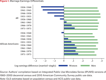
Differences in work behavior and earnings associated with marital status and the presence of children are well documented. In the cross-section, wage regressions typically find that married men earn from 10 percent to 40 percent more than single men (see, for example, Korenman and Neumark 1991; Antonovics and Town 2004). In contrast, married women earn significantly less than unmarried women with similar human capital characteristics, especially those with children (see, for example, Waldfogel 1997, 1998).1 Evidence indicates that two patterns contribute to these differentials: first, selection, by which we mean that characteristics related to earnings differ between those who are married and those who are not; and, second, specialization, in which spouses increase total family consumption when one spouse invests more heavily in skills rewarded in the labor market and the other takes a primary role in home production. We expect specialization to lead to faster wage growth relative to single peers for one spouse, but a decline relative to peers for the other. For example, Sanders Korenman and David Neumark (1991) find evidence of positive selection of men into marriage based on earnings—that is, men with higher earnings are more likely to marry. But they also find that much of the marriage premium accrues from faster wage growth for men after marriage, which is consistent with marriage allowing men to shift toward more market work and less home production.2 Comparing married and cohabitating couples in Sweden, Donna Ginther, Marianne Sundstrom, and Anders Bjorklund (2008) find that most of the marriage premium among men can be attributed to positive selection while increased specialization after marriage accounts for the marriage penalty for women.3 How have earnings differentials associated with marriage—which we refer to as marriage gaps—evolved over time? Figure 1 presents estimates of these gaps for cohorts born between 1936 and 1975 based on a series of cross-sectional surveys.4 In the cross-section, married men enjoy a substantially positive earnings gap, on the order of 30 to 35 log points, that has remained fairly stable across these cohorts. Married women, on the other hand, began with a substantially negative earnings gap (-24 log points for the 1936 to 1940 cohort) but across cohorts have steadily gained relative to their single counterparts. In the most recent birth cohort (1971 to 1975), married women enjoy a positive earnings gap of 11 log points. The trend among black women is similar but the change is not as dramatic, the gap changing from roughly -3 log points for the 1936 to 1940 cohort to positive 15 log points for the most recent cohort.
Marriage Earnings Differentials
Betsey Stevenson and Justin Wolfers (2007) hypothesize that the returns to marriage based on production complementarities have diminished over time. The introduction of technology in household production, such as washing machines, vacuum cleaners, and microwave ovens has reduced incentives to marry based on household specialization (Greenwood and Guner 2008). Women's market opportunities increased for a variety of reasons, making it more costly for women to stay home. In addition, unilateral divorce laws also increased the risk associated with specializing in the household sector for women (Stevenson 2007). Although the returns to specialization may have declined, the benefits of marriage based on consumption and leisure complementarities may have increased with increased longevity and leisure (Aguiar and Hurst 2007). Based on these developments, we would expect to find that the marriage gaps for both men and women have narrowed over time.5
The factors that led to declining marriage rates, however, did not affect all men and women equally. Although wages of women in general rose relative to those of men, the gains were larger at the bottom of the skill distribution than at the top (Blau and Kahn 1997). Among less-educated couples especially, the incentive to marry based on household specialization fell as male earnings prospects fell. Evidence is considerable that these changes resulted in shifts in selection into marriage as well. Among women, the cross-sectional correlation between marriage and education has reversed sign. In earlier cohorts, marriage rates were lowest among the most-educated women, whereas now the most-educated women are the most likely to be married (Isen and Stevenson 2010; Goldstein and Kenney 2001). Among men as well, marriage rates have fallen most dramatically for the less educated, reinforcing the positive relationship between marriage and earnings potential in earlier cohorts.
In this study, we examine how these shifts have affected the evolution of earnings differentials associated with marriage and the importance of selection versus specialization in understanding these changes. Our basic empirical strategy is to estimate marriage gaps in earnings using both ordinary least squares (OLS) and fixed-effects (FE) models. OLS estimates combine the effects of changes in earnings associated with a change in marital status (specialization) with any persistent existing differences in mean earnings between those who are married and those who are not (selection effects). When we include fixed effects, the coefficient on marriage isolates changes in earnings associated with a change in marital status. Our specifications include controls for age, so where our FE estimates show negative marriage gaps for women, this reflects slower wage growth for women relative to their peers during periods when they are married. The difference between the two estimates then provides us with the net effect of selection into marriage. We use data from Survey of Income and Program Participation (SIPP) panels matched to Social Security Administration (SSA) earnings records from 1954 to 2011. These data have many advantages for our purposes: they provide detailed earnings histories that allow us to estimate both OLS and fixed-effect models of the marriage premium; the samples of individuals from the pooled SIPP panels are considerably larger than those available from other long panels such as the University of Michigan's Panel Study of Income Dynamics (PSID) or the National Longitudinal Survey of Youth 1979 (NLSY79); and the earnings data span enough time to allow us to meaningfully compare across birth cohorts. Sarah Avellar and Pamela Smock (2003) conduct fixed-effects analysis to compare changes in the motherhood wage gap for two birth cohorts—NLS Young Women and the NLSY. Our paper examines both marriage and motherhood gaps and to the best of our knowledge, our paper is the first to compare OLS and FE models for birth cohorts spanning four decades. An important caveat is that we observe annual earnings but not hours worked in our data, and therefore we cannot separately examine the relative contributions of wages and hours. We do, however, examine the extent to which the earnings changes for women are driven by women leaving the labor force and having zero earnings.
To preview our findings, we find that selection into marriage has become increasingly positive: that is, higher levels of education and earnings potential are both associated with a greater likelihood of being married. Like Adam Isen and Betsey Stevenson (2010), we find that the most-educated women are the most likely to marry among the most recent birth cohorts. Pooling our sample of women born between 1936 and 1975, we find an average earnings gap of approximately -26 percent associated with marriage. The marriage gap is roughly half as large (-12 percent) when we control for the number of children and the presence of young children. Our estimates are somewhat more negative in fixed-effect specifications (-29 percent), indicating that positive selection into marriage leads to some understatement of the average marriage gap for women in our sample.
Comparing across cohorts, we find that the marriage earnings gap became less negative for women in both OLS and FE estimates. In both sets, married women who remain childless actually enjoy an earnings premium in the most recent birth cohort (born between 1966 and 1975). Among women with children, the difference between the earnings of married and single women also narrows. Comparing OLS and FE estimates, we find that increasingly positive selection into marriage contributes to the reduction in the marriage earnings gap in cross-sectional data. Our findings imply that marriage is no longer associated with lower earnings among women in the most recent cohort, but we find that the motherhood gap remains large.
We find quite different results for men. Although educated men with the highest earnings potential have always been the most likely to marry, the relationship has become more pronounced among recent birth cohorts. Pooling across all cohorts of men, we find a positive OLS estimate of the marriage earnings gap of approximately 34 percent. In FE specifications, however, the estimate is reduced by more than half, to about 14 percent, suggesting that selection plays an important role in accounting for the marriage premium for men. When we allow the premium to vary across cohorts, we find successively larger positive marriage gaps in the fixed-effect regressions. This would suggest an increase in specialization across successive birth cohorts. Such an interpretation, however, assumes no selection into marriage on wage growth. We suspect that this empirical regularity instead represents either selection on individual-specific earnings growth rates or an interaction between changes in age-earnings profiles and changes in patterns of selection into marriage. We have begun to investigate these possibilities but have not yet resolved this puzzle.
DATA
Our sample of individuals is drawn from respondents in the 1984, 1990 to 1993, 1996, 2001, 2004, and 2008 SIPP panels who provided the information needed to validate matches to Social Security Administration earnings records.6 Individuals had to be at least fifteen years old at the time of their second SIPP interview to be eligible for inclusion in the matched data.7 For matched individuals, we use annual earnings for 1954 through 2011 based on annual summaries of earnings on jobs recorded in the SSA Master Earnings File. The primary source of the earnings information is W-2 records, but self-employment earnings are also included. We include employees’ contributions to deferred compensation plans as part of our earnings measure. For the years prior to 1978, earnings measures are truncated at the maximum earnings subject to FICA (Federal Insurance Contributions Act) taxes. A significant number of men in our sample have earnings that exceed the taxable maximum, and so are understated in our data.8 But the cap affects only a small share of women in our sample, in part because our sample is young in those years, for example, age at most twenty-nine in 1965, the year in which the share of all covered workers who had earnings that exceeded the taxable max reached its peak of 36 percent.9 For both men and women, we use the full distribution of earnings for 1978 through 1990 to estimate the appropriate adjustment to log earnings based on the assumption that the upper tail of the earnings distribution resembles a Pareto distribution, and then use the parameter estimate to make a mean adjustment to log earnings for those affected by the cap.10 The small adjustment to earnings for women made little difference for any of our estimates, so we present those with the adjustment here. As expected, the adjustment had more important effects on the results for men, particularly for estimates of changes across cohorts, given that the earliest cohort was much more affected than later ones. So for men, the regression results we present here are based only on 1978 through 2011 earnings. Marital histories, educational attainment, and women's fertility histories are based on data collected in the SIPP. Age is based on SSA sources.
We use these data to look at cohorts born between 1936 and 1975, following their earnings over years in which we have earnings data, and the individual had one to thirty-five years of potential experience.11 To determine marital status at a given time, we use the marital history information collected in the relevant SIPP panel with some additional updates from changes in later waves of that panel. This largely gives us the information we need for years leading up to or during the SIPP panel, but not for the years after the panel is over. For this reason, we drop any earnings records from years after the individual is last observed in the panel. Because our focus is on marital status, we further restrict the sample to men and women who are interviewed at age thirty-five or older, so that at a minimum we know marital status through age thirty-five for everyone in the sample. Thus, for a fifty-year-old woman interviewed in the 1990 SIPP panel who did not start college, we use earnings for 1958 to 1992 (ages eighteen through fifty-two); and for a thirty-five-year-old college graduate interviewed in the 1996 panel, we use earnings for 1984 to 1999 (ages twenty-five through thirty-eight).
Table 1 presents descriptive statistics by birth cohort for the men and women in our sample. The first pair of panels (person-weighted) consists of variables that do not vary year by year, so each individual contributes a single observation. The second pair of panels is based on the full set of person-year observations we use in our regressions, so individuals who we follow for more years contribute more observations to the sample means.12 In general, the differences across cohorts in the top panels reflect well-established trends in the population: for example, the earliest cohort has less education and more children. We can, though, follow members of the older cohorts to later ages. This is why the sample mean of age is larger for the older cohorts. On the other hand, despite their higher fertility, women in the first cohort have lower means for time-varying child variables, such as having a child younger than six in the current year, as shown in the bottom panel.
Sample Means
TRENDS IN MARRIAGE RATES
We first examine who is married among men and women. In particular, we are interested in whether those with relatively high stocks of human capital are more or less likely to marry than the average person. A pattern of positive selection into marriage based on labor-market characteristics will tend to widen the gap in earnings of married couples relative to singles. We characterize labor-market skill in two ways—using education levels and using estimated potential earnings. Although education level is a relatively simple, clean measure, its distribution has shifted significantly over time and in different ways for men and women, making it more complicated to parcel out what represents a change in selection patterns and what is simply the result of shifting education distributions.
We construct a measure of potential earnings based on predicted earnings from a fixed-effect regression of log earnings on year dummies, main effects for education, a quartic in age, interactions between the age terms and education dummies, marital status, and for women, age and presence of children. We use the results to predict earnings for a single, childless person at age forty, and then add the estimated person-specific fixed effect to that prediction to get potential earnings.13 For the small portion of women in the sample who matched to the SSA earnings database but had zero earnings in all the years they were in the sample, we assign a random draw from the distribution of this measure. The random draw is taken from among other members of their birth cohort with the same education level who had relatively large numbers of years with zero earnings. We then assign each person to a potential earnings quartile based on their ranking among those of the same gender in their ten-year birth cohort. Although this measure will capture potential earnings imperfectly, it incorporates information drawn from the earnings data in addition to education level, and also has the advantage that we can use it to divide men and women into equal size groups over time.
Table 2 presents the share of men and women who are married at age thirty-five by level of education and by ten-year birth cohort. Overall, the probability of marriage fell between the 1936 to 1945 and 1956 to 1965 cohorts for all education groups, and for both men and women. Some evidence indicates a rise in the share married at thirty-five for the last birth cohort among college graduates, but the share married among those with less schooling continued to fall. Among men, the general pattern is that, with few exceptions, being married is positively associated with higher levels of education. Over time, however, marriage rates dropped more among the less educated, widening the gap across education groups. For women, marriage was modestly negatively associated with education in the first birth cohort, but a larger drop in marriage rates for the less educated resulted in a substantially positive relationship in the most recent birth cohort.
Marriage Rates, Age Thirty-Five
These changes in the relationship between the probability of marriage and education level resulted in a substantial decline in the education levels of single relative to married people, particularly for women. Reconfiguring the information in table 2, in the 1936 to 1945 birth cohort, single women were slightly more likely to be college graduates than married women (20 percent versus 19 percent), but by the 1966 to 1975 cohort, that pattern had reversed. Approximately 38 percent of married women were college graduates, but only 26 percent of single women were. For men, the change is less dramatic but still substantial: the share of college graduates grew 8 percentage points among married men but not at all among single men.14
This pattern of a shift toward those who are married being those with greater labor-market skills also appears in the statistics on marriage rates by quartiles of the potential earnings distribution, as illustrated in table 3. Again, overall the share of men and of women who are married at age thirty-five drops, but the decline in marriage is particularly large among those in the bottom part of the distribution. Comparing across the 1936 to 1945 and 1966 to 1975 birth cohorts of women, the share married increased slightly in the top quartile but fell 20 percentage points, from 0.80 to 0.60, in the bottom quartile. For men, the marriage rate in the top quartile declined 6 percentage points but 16 points in the bottom quartile. It is striking that in the most recent cohort only 55 percent of the men in the lowest earnings category are married at age thirty-five. Because the overall shares in these quartiles are fixed over time, these changes imply that marriage is becoming increasingly associated with better labor-market prospects. For men, this is a change in degree—married men are more educated and more likely to be in the upper part of the earnings distribution even in our earliest birth cohort, but the gap between married and single men increases over time. For women, negative selection into marriage on labor-market prospects was modest in the earliest cohort, but in our two most recent birth cohorts positive. Isen and Stevenson (2010) report similar changes in marriage patterns by education. Our analysis here using earnings percentiles confirm that the patterns reflect real changes in the selection into marriage, rather than shifting composition of education groups.
Marriage Rates at Age Thirty-Five, Potential Earnings Distribution
RELATIONSHIP BETWEEN MARRIAGE AND EARNINGS
Comparison of OLS earnings regressions with FE models is the basis of much of our regression analysis. To fix ideas, we start with the following stylized statistical model of earnings:
where i indexes an individual, C indexes birth cohort, j = m (male) or f (female), and X = observable characteristics such as education and age, M = marital status indicators, and K = indicators for the presence and age of children. In this specification, E(εjCi) + E(νjCit) = 0, αjCi = permanent (unobserved) skill component of earnings and νjCit = transitory shocks. Adding interaction terms between M and characteristics of the individual allows us to examine how the marriage gap varies with these characteristics. We also include analogous interactions between K and individual characteristics in this part of the analysis.
Our first step is to examine changes in average differences in earnings associated with marital status, which are measured by γjC. We run the regressions for men and women allowing for differences across birth cohorts. We first estimate the earnings regressions via ordinary least squares, in which case the marital status and parenthood coefficients include selection effects—that is, they confound changes in earnings with marriage-children with average differences in the permanent skill component (αjCi) associated with marriage and children. We then estimate the regressions using fixed person effects in an attempt to remove effects of selection on earnings levels.15 The FE marriage earnings gap captures the average difference in an individual's earnings between periods in which they are married and those in which they are not, relative to the average age-earnings profile. These are our estimates of the effects of specialization, by which we mean changes in earnings that arise from changes in work behavior that result from marriage. The difference between the OLS and FE estimates provides us with an estimate of the net effects of selection on these differentials. That is, the difference gives us an estimate of the extent to which the earnings of those who are currently married are persistently different from the earnings of those who are currently single.16
MARRIAGE AND WOMEN'S EARNINGS
Table 4 presents coefficient estimates from the earnings regressions for women. In column (1) we report the coefficient on the “married” dummy without controlling for children and in column (2) we control for the number of children and whether any of those children are younger than six.17 In column (3), we interact both married and children dummies with birth cohort to estimate the evolution of marriage and child effects on earnings. Finally, in column (4), we additionally interact the married and children variables with each other and with birth cohort dummies, thereby allowing the impact of children on earnings to differ between married and single women, and for that interaction effect to vary across cohorts.
Log Earnings Regressions, Women
We find a substantial negative earnings differential for married women in the first specification for both OLS and FE estimates. The larger absolute size of the fixed-effect estimate implies that, for this set of cohorts overall, positive selection into marriage offsets a modest share of the differential. That is, pooling all of our data, the negative changes in earnings profiles associated with marriage are slightly larger than the average difference in earnings between married and single women because women with higher earnings are slightly more likely to be married. Consistent with others’ findings, adding controls for children in column (2) reduces the marriage differential substantially. In the OLS regression, the marriage earnings differential falls by more than half, from –0.256 to –0.118. In the FE regression, the coefficient falls by about one-third, from –0.292 to –0.197.
In column (3), we add interactions between the married and children variables and ten-year birth cohort dummies to examine changes in these earnings differentials across these cohorts of women. In both the OLS and FE regressions, the earnings differential associated with marriage becomes less negative across birth cohorts. The decline in the earnings differential in fixed-effect estimates suggests a much reduced role for specialization. Comparing the OLS and FE estimates, we find a larger increase between the earliest and the most recent birth cohorts in the OLS estimate (0.331) than in the FE (0.277). This implies that selection into marriage based on potential earnings became increasingly positive across these cohorts—that is, women with higher potential earnings became more likely to marry. The finding of positive selection into marriage on earnings characteristics is quite consistent with the evidence we present in table 2, and also with the findings of Isen and Stevenson (2010) on selection based on education. In contrast to the consistent shrinkage of the marriage differential across these cohorts, the coefficients on the children-cohort interaction terms do not show a notable decline in the earnings differentials associated with children. The differential associated with young children has declined across cohorts but the differential associated with school-age children has actually increased.
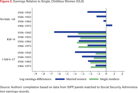
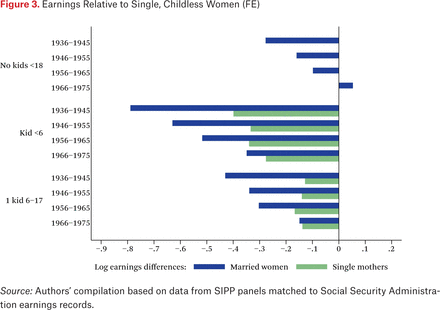
In the final specification in (4), we also include three-way interactions that allow the earnings differentials associated with children to differ between married and single women, and for that to vary across cohorts as well. The three-way interactions make it much more difficult to interpret individual coefficients, so we present a series of earnings differentials in figures 2 and 3 that describe the patterns of interest: figure 2 based on the OLS results, and figure 3 on our FE estimates. Each estimate in the figures gives an earnings differential for a particular group based on specification (4) relative to single, childless women in the same cohort. To illustrate how changes across cohorts in the marriage differential differ between women with children and those without, we include implied differentials for two child scenarios—having one school-age and having one preschool-age child.
Earnings Relative to Single, Childless Women (OLS)
Earnings Relative to Single, Childless Women (FE)
The more heavily shaded bars in the graphs represent differentials for married women, and the lighter ones indicate those for single women. The top panel gives the marriage differential for women without children, and in both figures this differential is positive for the most recent cohort. In other words, among the most recent birth cohort of women who remain childless, marriage actually increases earnings relative to single women without children.18 The second and third panels give estimated differentials for married and single women with one preschool aged child and one school-age child respectively. In both the OLS and FE results, we see little change in the earnings of single mothers relative to single, childless women, but large decreases relative to that group for married women with children.
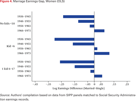
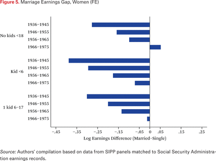
The marriage differential in these figures, conditional on children, is given by the difference between the married and single bars and we present this differential in figures 4 and 5. Both the OLS and FE estimates imply that the gap in earnings between married and single women with children has declined dramatically. The OLS results (figure 4) suggest that married women with children now earn more than single women with children, but comparison with the FE results (figure 5) suggests that this is due to married women with children being increasingly positively selected relative to single women with children. In FE estimates shown in figure 5, we find that the motherhood wage gap is larger for married women than single women. Michelle Budig and Paula England (2001) and Alexandra Killewald and Margaret Gough (2013) find similar results using the NLSY79 data. They interpret these results as being consistent with the motherhood wage gap being augmented by specialization between married parents.
Marriage Earnings Gap, Women (OLS)
Marriage Earnings Gap, Women (FE)
Although our findings imply that marriage is no longer associated with lower earnings among women in the most recent cohort (with the exception of married women with young children who are still slightly behind their single counterparts), it is important to keep in mind that the motherhood gap (as shown in figure 3) remains substantial. Even among the most recent birth cohort, married women with preschool-age children have approximately 35 percent lower earnings than married women without children and that married women with school-age children have approximately 15 percent lower earnings. These findings are broadly consistent with Avellar and Smock (2003), who find that in fixed-effects regressions the motherhood wage gap had not diminished across two recent cohorts—NLS Young Women and the NLSY.
MARRIAGE AND WOMEN'S PARTICIPATION
These log earnings results condition on having positive earnings. We cannot separately examine wages and hours worked in our data, but we can examine changes in women's entering or leaving the labor force and having positive versus zero earnings. To look at this extensive margin, we estimate specifications similar to (1) but with an indicator for having positive earnings in a calendar year as the dependent variable.19
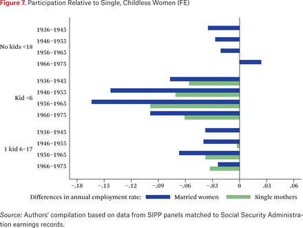
The results of the regressions are reported in table A1 but we illustrate changes in the participation gap associated with marriage and motherhood in figures 6 and 7 (showing OLS and FE estimates respectively). Like figures 4 and 5, these are based on specifications in which we allow for interactions between marriage and children that change across cohorts. In both figures, we see that the participation differential between married women without children and single women without children declined so that married women are in fact slightly more likely to participate than single women among the most recent birth cohort. In contrast, the participation differential between married mothers and single mothers remains negative and shows no clear pattern of decline. Mothers with young children in particular continue to participate substantially less than single and married women without children. Our results on the participation effect of young children are broadly consistent with Byker (this volume) who also does not find much trend across cohorts in changes in mother's labor force participation around the time of birth.
Participation Relative to Single, Childless Women (OLS)
Participation Relative to Single, Childless Women (FE)
MARRIAGE AND WOMEN'S EARNINGS BY EDUCATION AND RACE
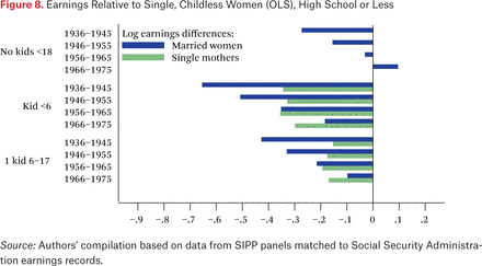
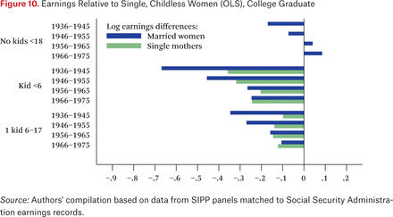
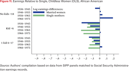
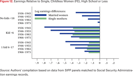
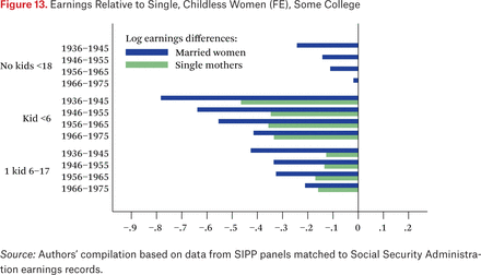
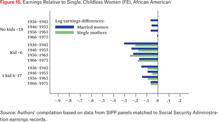
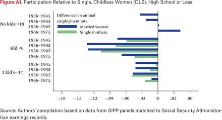
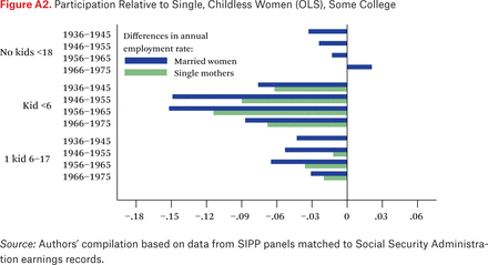
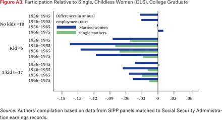
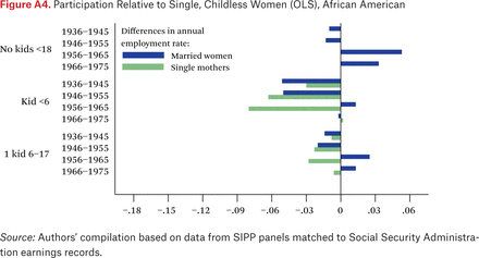
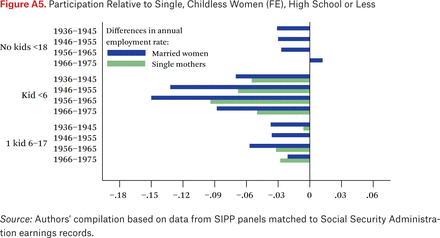
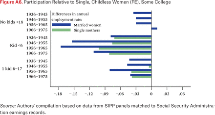
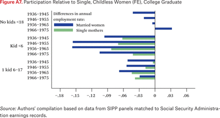
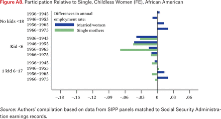
Finally we explore the effect of marriage on women's earnings by education groups and also separately for African American women. We report the regression results in table A2 but highlight the trends associated with the fully interacted model in figures 8 through 11 and 12 though 15. We find patterns similar to those in the overall changes when we disaggregate by education group and race, with the exception of college educated women. Looking first at the OLS estimates shown in figures 8 through 11, we find that the earnings differential associated with marriage becomes less negative. These changes are larger in the OLS estimates than the corresponding FE estimates shown for women without a college degree (figure 12) and for black women (figure 15). It appears that among these groups, women with higher earnings potential were increasingly more likely to marry, suggesting that selection plays an important role. Changing selection is less evident among female college graduates. For example, among women without children, the 1966 to 1975 cohort of married women have higher earnings relative to single women in OLS estimates. For less-educated women, this positive earnings differential disappears in FE estimates, suggesting that positive selection played a role. Among college graduate women, however, the positive earnings differential remains even in FE estimates.
Earnings Relative to Single, Childless Women (OLS), High School or Less
Earnings Relative to Single, Childless Women (OLS), Some College
Earnings Relative to Single, Childless Women (OLS), College Graduate
Earnings Relative to Single, Childless Women (OLS), African American
Earnings Relative to Single, Childless Women (FE), High School or Less
Earnings Relative to Single, Childless Women (FE), Some College
Earnings Relative to Single, Childless Women (FE), College Graduate
Earnings Relative to Single, Childless Women (FE), African American
MARRIAGE AND MEN'S EARNINGS
Table 5 presents estimates of the marriage premium for men based on the same log earnings regressions we estimated for women except that we do not control for children.20 We find a very large positive marriage premium for men in the pooled regressions, but the fixed-effect estimates are much smaller. This is consistent with our findings in tables 2 and 3 that selection on labor-market skills into marriage is quite positive for men. The estimated interaction effects with birth cohort dummies are somewhat puzzling. They indicate that the FE marriage premium has risen steadily across cohorts. The OLS estimates have risen as well, but have done so more slowly and less consistently. The large increase in the marriage premium over time in the FE results suggests that selection into marriage has declined somewhat in importance, and that the effects of specialization after marriage have increased. That seems inconsistent with both the increase in the selectivity of marriage for men—documented in tables 2 and 3—and with evidence of increased labor-market skills and work among married women across these cohorts. When we allow the marriage premium to vary with education level (table A4), the OLS and FE results similarly imply a reduction in selection but growth in specialization for each group of men we examine.
Log Earnings Regressions, Men
One possibility is that the fixed-effect estimates for early cohorts of men are downward biased because we have earnings for them only at older ages. For example, for those born in 1936, we observe earnings beginning at age forty-two, long after most would have married. Thus changes in marital status for this group are likely to involve primarily divorce and remarriage which might have smaller effects on earnings than first marriages. But our OLS estimates for men based on public-use data in figure 1 also show an inconsistent rise in the marriage gap for men. It is also possible that our implicit assumption of constant returns to experience over time is leading to a rising estimate of the marriage premium in both the fixed-effect and pooled results because married men on average have greater experience than unmarried men. However, examination of alternative specifications in which we allow returns to experience and education to change over time leads to essentially the same pattern as in the results presented here. A third possibility is that some selection into marriage is based on individual-specific earnings growth, in which case the fixed-effect estimates are also subject to bias from selection. Given such a misspecification, changes in the distribution of the individual-specific growth component, or in selection based on that component, could result in the pattern we find here.
CONCLUSION
We find that those who are married have become increasingly positively selected from the population at large in terms of both education and earnings potential. Consistent with other studies, we find that the most-educated women are the most likely to be married among recent birth cohorts. Although educated men with the highest earnings potential have always been the most likely to be married, the relationship has become more pronounced across birth cohorts spanning 1936 to 1975.
How has this increased selection affected male and female marriage gaps? Among women born between 1936 and 1975, we find an average earnings gap of approximately 26 percent associated with marriage that falls to 12 percent when we control for children. Our fixed-effect estimates are somewhat larger, at 29 percent, indicating a slight positive selection into marriage overall. Comparing across cohorts, we find that the marriage earnings gap fell for women both in the cross-section and in fixed-effect estimates. In both the OLS and FE estimates, married women who remain childless actually enjoy an earnings premium in the most recent birth cohort—women born between 1966 and 1975. Among women with children, the difference between the earnings of married and single women also narrows. Our findings imply that marriage is no longer associated with lower earnings among women in our most recent cohort, but the motherhood gap remains large. In contrast to the consistent shrinkage of the marriage differential across these cohorts, the coefficients on the children-cohort interaction terms do not show a notable decline in the earnings differentials associated with children.
Our results are somewhat at odds with Pal and Waldfogel (this volume), who find a decline in the overall motherhood wage gap in the more recent period, from 1993 to 2013. One potential explanation for the differences in our findings is that they focus on hourly wages rather than annual earnings. They also include more recent birth cohorts at younger ages, which may put more weight on the motherhood gap associated with having young children. We also find that the motherhood gap associated with young children has decreased.
Comparing OLS and fixed-effect estimates, we find that increasingly positive selection into marriage contributes to the reduction in the marriage earnings gap measured in cross-sectional data. Particularly for mothers of preschool-age children, OLS estimates are somewhat misleading in that marriage continues to be associated with a reduction in earnings growth relative to peers that we associate with household specialization.
We find quite different results for men. We find an OLS estimate of the marriage earnings premium equaling 34 percent for men. In FE results, however, the estimate is reduced to less than 14 percent, suggesting that selection plays a much more important role in accounting for the positive marriage gap for men. In specifications that allow marriage to affect only the level of male earnings, we find successively larger marriage premiums in the FE regressions. Taken literally, this would suggest an increase in specialization across successive birth cohorts. We suspect that instead this represents some form of misspecification. We have begun to investigate these possibilities but have not yet resolved the puzzle.
Acknowledgments
Any opinions and conclusions are those of the authors and do not necessarily represent the views of the U.S. Census Bureau, the SSA, the NBER, or any other agency of the federal government. All results have been reviewed to ensure that no confidential information is disclosed. This research was supported by the U.S. Social Security Administration through Grant #NB10–10 to the National Bureau of Economic Research (NBER) as part of the SSA Retirement Research Consortium. We would like to thank Martha Bailey, Thomas DiPrete, and other participants of the Russell Sage conference “Changing Roles and the Status of Women,” and Martha Stinson for helpful comments. We also thank Gary Benedetto and Martha Stinson for help in using the data.
APPENDIX
Participation Regressions, Women
Log Earnings Regressions, Women
Participation Regressions, Women
Log Earnings Regressions, Men
Standard Errors for Table 4
Standard Errors for Table A1
Standard Errors for Table A2
Participation Relative to Single, Childless Women (OLS), High School or Less
Participation Relative to Single, Childless Women (OLS), Some College
Participation Relative to Single, Childless Women (OLS), College Graduate
Participation Relative to Single, Childless Women (OLS), African American
Participation Relative to Single, Childless Women (FE), High School or Less
Participation Relative to Single, Childless Women (FE), Some College
Participation Relative to Single, Childless Women (FE), College Graduate
Participation Relative to Single, Childless Women (FE), African American
FOOTNOTES
↵1. Fixed-effects models using data from the National Longitudinal Survey of Youth (NLSY79) find that for women, marriage, absent children, is positively associated with wages (Budig and England 2001; Killewald and Gough 2013). These results are consistent with what we find for the most recent birth cohort.
↵2. Christopher Dougherty (2006) finds that among men in the NLSY79, wages rise at least five years prior to marriage. This is still consistent with specialization if men invest in steady work and higher paying jobs in anticipation of marriage. On the other hand, it could also be consistent with selection into marriage based on time-varying shocks rather than persistent earnings differences. A simple fixed-effects model would not be able to disentangle the two channels in this case.
↵3. Another important explanation which we do not address in our paper is discrimination by employers. Conducting a laboratory study, Shelley Correll, Stephen Bernard, and In Paik (2007) find that subjects penalize mothers in terms of perceived competence and recommended starting salary. Part of what we attribute to specialization may be due to statistical discrimination as employers infer actions of individual men and women based on group characteristics.
↵4. The figure is based on 1960 through 2000 decennial census and 2010 American Community Survey's Integrated Public Use Microdata Series (IPUMS) data. The figure reports coefficients on five-year birth cohort dummies interacted with a currently married dummy from a regression of log annual wage and salary earnings on year dummies, a quartic in age, education dummies, number of children, and presence of children younger than five. The sample consists of men and women who have one to thirty-five years of potential work experience.
↵5. Some evidence indicates that the male marriage premium narrowed in the 1970s and 1980s (Gray 1997; Blackburn and Korenman 1994). Jeffrey Gray (1997) finds that the marriage premium fell, particularly for men whose wives work.
↵6. The results presented here are based on confidential data from version 6.0 of the SIPP Gold Standard File. External researchers can access related data through the public-use SIPP Synthetic Beta (SSB) files, and census staff will validate results obtained from the SSB on the internal, confidential version of these data (the Completed Gold Standard Files). For more information visit https://www.census.gov/programs-surveys/sipp/guidance/sipp-synthetic-beta-data-product.html.The U.S. Census Bureau also supports external researchers use of some of these data through the Research Data Center network (http://www.census.gov/ces/rdcresearch).
↵7. The SIPP is a series of short panel surveys in which respondents are surveyed every four months to collect detailed information on household members’ income, employment, and program participation over the previous months (for an overview, see http://www.census.gov/hhes/www/sippdesc.html). The surveys also periodically collect detailed information on the demographic characteristics and relationships of household members. Panels have ranged in length from about two to four years. Because our sample pools data from several SIPP panel samples, we do not use SIPP survey weights in our analysis, so the results cannot be assumed to be nationally representative.
↵8. In the late 1950s and early 1960s, more than 25 percent of covered workers had earnings that exceeded the taxable maximum in several years (see Whitman and Shoffner 2011).
↵9. Women may be more affected by the pre-1978 absence of earnings records in these data for workers who were not subject to FICA taxes, given that the excluded group included many public school employees. This will bias our estimates for the earliest cohorts if the relationship between earnings and marital status for this group differs from that among the women we do observe.
↵10. We estimate separate parameters for men and women, by year and by education group (high school diploma or less than high school versus college degree or some college). For women, the estimates are similar across education groups, so we use an adjustment on estimates that pooled the two groups. For men, the implied adjustment for the more educated group was substantially larger, so we apply it separately by education group. For both men and women, the estimated adjustment parameter does not vary much across years. Marriage premium estimates based on the 1954 through 2011 time series, using the capped data as is, yields somewhat smaller estimates of the marriage premium for men, but a larger increase across cohorts. This simply reflects that married men are more likely to have earnings that exceed the cap, so ignoring the truncation understates the marriage premium in early cohorts. Using the mean adjustment based on the Pareto distribution results in noisier fixed-effect estimates.
↵11. Specifically, for those who finished high school or less, the age range is eighteen to fifty-three. For those with some college, the range is twenty-one to fifty-six. For college graduates, the range is twenty-three to fifty-eight. For those with postcollege education, it is twenty-five to sixty. We drop the very small share of men for whom we never observe positive earnings but keep women with no earnings because we estimate participation regressions for women but not men.
↵12. Sample counts are rounded to the nearest hundred here to help maintain respondent confidentiality. Person-year counts include all years in the window over which we have data for the individual, whether or not earnings are observed in a particular year.
↵13. This measure is essentially based on average earnings that have been adjusted for differences in age, calendar years observed, marital status, and for women, presence and age of children using the regression coefficients.
↵14. For men, the share of college graduates does not consistently grow across each of these birth cohorts. The sharp increase and then decline over the first three cohorts of men likely reflects the effect of Vietnam-era draft deferrals on men's college attendance documented in David Card and Thomas Lemieux (2000), which was greatest for men born in the late 1940s. We focus on the increase from the first to the last cohort as reflecting the longer-term trend increase in college attendance.
↵15. This method interprets steeper wage growth among married men as an effect of marriage, but it is difficult to entirely rule out selection because men with higher expected wage growth may be more likely to marry.
↵16. Our specifications implicitly assume that divorce is associated with the same absolute change in earnings as marriage, but with the opposite sign. We examine specifications that allowed these effects to differ but find that this simplification is a reasonably good description of the patterns in our data.
↵17. In our specification, we cap the number of children at three because in specifications in which we use a series of dummy variables to control for children, additions beyond three had little additional effect on our estimates. The count of children younger than eighteen includes those younger than six, so the coefficient on the count of children younger than eighteen represents the effect of one school-age child and that on the dummy for having a child younger than six gives the additional effect of having that child be preschool age. We use information from fertility histories to measure the number and ages of children. These questions apply only to biological children, and we know the year of birth for only the oldest and youngest children. We therefore miss the presence of all step- and adopted children. To create controls for children, if there are one or two biological children, we assume that both live with their mother between birth and the year they turn eighteen and set the control for the presence of young children based on the years in which one or both children were younger than six. For mothers with three or more children, we assume that a child younger than six was present between the sixth birthday of the first child and the birth of the last child. We count the number of children present between the birth of the first and of the last by assuming that the intervening child or children are evenly spaced. These measures are clearly approximations with errors in both directions—not all children are counted, but some of those who are counted do not live at home.
↵18. That this is also true for the fixed-effect estimates suggests that this is not due to selection on earnings levels. Both Alexandra Killewald and Margaret Gough (2013) and Michelle Budig and Paula England (2001) report similar results using the National Longitudinal Survey of Youth (NLSY79). One possibility is that women are increasingly likely to marry upon finishing college so that we observe their earnings rise along with change in marital status. When we disaggregate by education group, we find that the marriage premium for women without children among the recent birth cohort is due to women with a college degree.
↵19. Note that the estimates for the first two cohorts are likely to be affected by the exclusion of those not subject to FICA taxes in years prior to 1978.
↵20. We omit controls for children mostly because in the fertility history SIPP only collects a count of total number of biological children for men. Although we could put together information on the age and presence of children during the SIPP panel, doing so would miss the grown children of older respondents.
- Copyright © 2016 by Russell Sage Foundation. All rights reserved. Printed in the United States of America. No part of this publication may be reproduced, stored in a retrieval system, or transmitted in any form or by any means, electronic, mechanical, photocopying, recording, or otherwise, without the prior written permission of the publisher. Reproduction by the United States Government in whole or in part is permitted for any purpose. Any opinions and conclusions are those of the authors and do not necessarily represent the views of the U.S. Census Bureau, the SSA, the NBER, or any other agency of the federal government. All results have been reviewed to ensure that no confidential information is disclosed. This research was supported by the U.S. Social Security Administration through Grant #NB10–10 to the National Bureau of Economic Research (NBER) as part of the SSA Retirement Research Consortium. We would like to thank Martha Bailey, Thomas DiPrete, and other participants of the Russell Sage conference “Changing Roles and the Status of Women,” and Martha Stinson for helpful comments. We also thank Gary Benedetto and Martha Stinson for help in using the data. Direct correspondence to: Chinhui Juhn at cjuhn{at}uh.edu, University of Houston, Department of Economics, 3623 Cullen Boulevard, Room 204, Houston, TX 77204–5019; and Kristin McCue at kristin.mccue{at}census.gov, U.S. Census Bureau, CES/2K130E, 4600 Silver Hill Rd., Washington, D.C. 20233–6300.
Open Access Policy: RSF: The Russell Sage Foundation Journal of the Social Sciences is an open access journal. This article is published under a Creative Commons Attribution-NonCommercial-NoDerivs 3.0 Unported License.


