
Abstract
Population and housing growth are closely linked in the U.S. Census, less so in analysis. Overlooked changes in cohort size and lagged measurements have misled about current housing preferences, and quantity of housing needed, with mistiming producing great volatility. Drawing on decennial census data and American Community Surveys, we develop a cohort-based housing lifecycle model measuring active household formation of renters and owners in intervals from 1990 to 2021. Restrictions of credit and supply legislated in 2010 were aimed at curbing the excesses of the early 2000s bubble but clashed after 2011 with requirements of much larger millennial cohorts, creating shortages in rentals, then ownership. Cohort advancement through the housing lifecycle was greatly delayed until after 2016, when substantial catch-up began of postponed homeownership, widely varied by race. Housing policy should anticipate housing needs of changing cohort sizes and expected life-course transitions, reducing long lags between supply and demand.
Population and housing are intimately linked in family life and in the U.S. Census of Population and Housing. Fully 97 percent of the population lives in housing units, and the very identification and count of households is registered by presence of occupied housing units. Despite the joint collection of data about the population and housing universes in the census and the American Community Survey (ACS) and other major surveys, relatively little research attention has been given to interactions of the two universes. More than just correlating current characteristics of housing and its occupants, population and housing are both subject to long legacy and lag effects that require a deeper integration in order to explain and reduce their frequent misalignment.
Events of the early twenty-first century have cast harsh light on the neglect of both housing’s connection to a prospering economy and its vital support of family life and population growth. The global financial crisis and Great Recession were precipitated by a bubble in U.S. housing prices, whose collapse then undermined the entire financial system, with effects lingering more than a decade after. As a result, the American public—especially the younger generation and people of color—has borne the brunt of acute housing shortages, lack of affordability, and falling homeownership.
The decennial census is an opportunity to overview the changing linkage of housing and population, and to seek better insight on how underlying, major forces have precipitated so many undesired trends. Aided by annual observations of the American Community Survey, we have been studying the pace of post-2010 housing recovery, tracking both supply and demand, and giving special attention to the millennial generation that is both fueling growth in demand and bearing the brunt of current housing shortfalls (Myers, Lee, and Simmons 2020; Myers, Park, and Cho 2021). New work developed here delves deeper into major faults in key indicators traditionally used to measure linkage of population and housing. Beginning in the 1990s, and then spilling into volatile periods of boom, bust, and sustained housing shortage, policymakers and housing analysts appear to be misled about crucial linkages of demographic change to housing demand. We argue, in essence, that the 2000s decade of ample supply of housing and loose mortgage credit was built on a base of shrinking demographic demand, but following the collapse, policy and institutional response in the next decade erred in the opposite direction—namely, constricting construction and tightening financing in ways ill-designed for the swelling demand of the large millennial generation.
DEEP BUT LAGGED CONNECTIONS OF HOUSING AND POPULATION
Housing and population have a deep practical connection, given that the vast majority of people reside in housing units, often for decades in the same house, which leads to the joint collection of housing and population data in the decennial census and major surveys by the Census Bureau.1 The major nexus between population and housing is the household, defined as the group of people, or single individual, that occupies a housing unit. However, a key difference centers on the universes that provide the denominators for characteristics or behaviors, whether the question is one about housing characteristics of the population base or, alternatively, the population characteristics of the housing base.
The subfield of housing demography adopts a more conscious versatility in switching between population and housing denominators, and it invites the time-honored question, what comes first, population or housing (Myers 1990)? The causal order reverses between levels of geography and for different questions. At the local level, housing must be built before it can be occupied by people, and once built, it is virtually permanent in place, so people come and go, passing through the housing unit. However, at the regional or national level, it is population growth that creates the demand for housing to be built in the first place. And, even prior to that, it is the fertility of earlier decades that creates the wave of people, such as millennials, who will sweep into household forming ages (augmented by immigrants) and require housing.
Denominators in housing research typically are restricted to either households or housing units, rarely extending to the population base that forms the households for analysis (but see Lee and Painter 2013; Paciorek 2016). The population base integrates with the most widely provided data for tracking past and future growth—namely, total population and age groups. For long-term analysis, a population base holds crucial advantages.
Integration of demographics with housing demand analysis has the further advantage that the field of demography brings a focus on multiple dimensions of time that shape supply and demand. All demographic analysis is in units of time—age, birth years, durations, and periods. In theory and evidence to follow, this temporal perspective helps address housing change on several interacting time dimensions. A primary analytical tool is to convert ages to cohorts whose cumulative housing legacies can be tracked through time. The aggregated grouping of a cohort holds major advantages over age groups that are disconnected from the prior histories of the people currently occupying each age group.2 In particular, cohort analysis enables better tracking of lagged effects in groups of consumers’ lives.
Simple Mismatch of Housing and Population Growth
Surface indicators suggest how mismatched is the growth of housing and population. A century-long trend has found ever smaller average household sizes, falling from 3.33 in 1960, at the height of the baby boom, to 2.76 in 1980, and declining to 2.55 by 2020 (U.S. Census Bureau 1983, 2023a; Fry 2019). Fully one-quarter (27.6 percent) of occupied units in 2020 had a single person residing and well over half (60.5 percent) of all housing units (58.4 percent of owner-occupied) had only one or two occupants (U.S. Census Bureau 2023a). Yet at the same time that small households predominate, the percentage of single-family homes newly built with four bedrooms or more has risen from 20 percent in 1980 to 48 percent in 2022, and the share with at least three bathrooms has risen from 24 to 64 percent in the same period (U.S. Census Bureau n.d.-b).
The greatest mismatch today is affordability given that the prices of owned homes and rents have increased much more rapidly than incomes. In real terms, median home values increased 68.3 percent between 1980 and 2022 and median gross rents by 32.7 percent, but median household income increased only by 10.1 percent.3 Thus, households have had to allocate larger shares of budgets to housing expenses. Indeed, younger households in particular leverage their income much more highly to achieve homeownership, with three times the income elasticity among those of age thirty than at age fifty (Gabriel and Rosenthal 2015, figure 3a). In addition, young homebuyers are more likely to depend on parental assistance for down payments (Lee et al. 2020).
Temporal Lags Endemic to Housing Linkages with Population
A key feature linking population and housing more deeply in census data is shared core temporal properties.4 Housing’s unique feature recognized among consumer products is its great durability and expense, which requires reliance on long-term finance for its purchase. A further feature of housing is the length of time required to plan and carry out new construction, so supply changes typically lag two or more years behind changes in demand, which causes demand to periodically overheat available supply.
Population change might appear to proceed gradually, but key consumer decisions are bunched in a fairly narrow portion of the lifetime, ages twenty to forty. Nonetheless, people’s housing consumption changes can be held back by volatile economic events of rising interest rates or recession, subsequently with pent-up demand fulfilled when opportunities are more accommodating. As a result, housing changes have been anything but gradual.
The following temporal dynamics are fundamentals called out for attention and are invoked in later assessments of the housing bust, recovery, and shortages.
Young Adults Move at High Velocity but Older Adults Are Long Settled
Young people change residence frequently after completing their education, but in their mid-twenties begin to make increasingly long-term residence decisions. The census asks how long the household has lived in their current residence, and those data are highly revealing of consumers’ growing length of association with their current residence (table 1). The vast majority of young householders (under age thirty-five) are recent occupants who have resided in their current housing unit for less than five years, and many fewer older householders report themselves as having recently moved. Instead, half or more of older homeowners have lived continuously in the same home for more than twenty years. A particular implication of this length of occupancy is that the vast majority of occupants other than young renters have not recently selected their units; instead, they chose units to meet their current needs of a decade earlier or before, continuing their residence in the present home for reasons of sentiment, convenience, or simple inertia.
Length of Housing Occupancy, by Tenure, 2021 (Percentage of Age Group)
Homeownership Rates Are Compiled Through Past Accumulation
The length of housing careers creates a number of inconsistencies in current measurements. One of the most important, yet widely overlooked, is that the rate of homeownership largely is accumulated from purchase moves over many prior years. The high homeownership rates common among older homeowners, greater than 75 percent of households after age fifty-five, were accrued decades earlier. Referring again to table 1, half of such owners have not moved in the last twenty years, meaning that half at least were already homeowners twenty years earlier (in 2001, when they would have been between thirty-five and fifty-four). Further, many likely were repeat homebuyers at that time who first acquired homeowner status even ten years before that. Thus we should recognize that current homeownership is an accumulated status from the past, purchased at lower prices prevailing in earlier decades, not a current achievement paid through current income.
Homeownership Rates Are Lagged and Mislead About Current Preferences
The corollary of this long accumulation and persistence of homeownership rates is that current homeownership rates do not closely reflect trends in current desires or capacities for homeownership. A clear example emerged in the aftermath of the Great Recession. Between 2006, marking the end of the housing bubble, and 2015, the homeownership rate of young adults fell markedly,5 all the while serving as a centerpiece for popular narratives about generational failure and abandoned preferences for homeownership or actual purchase activity.
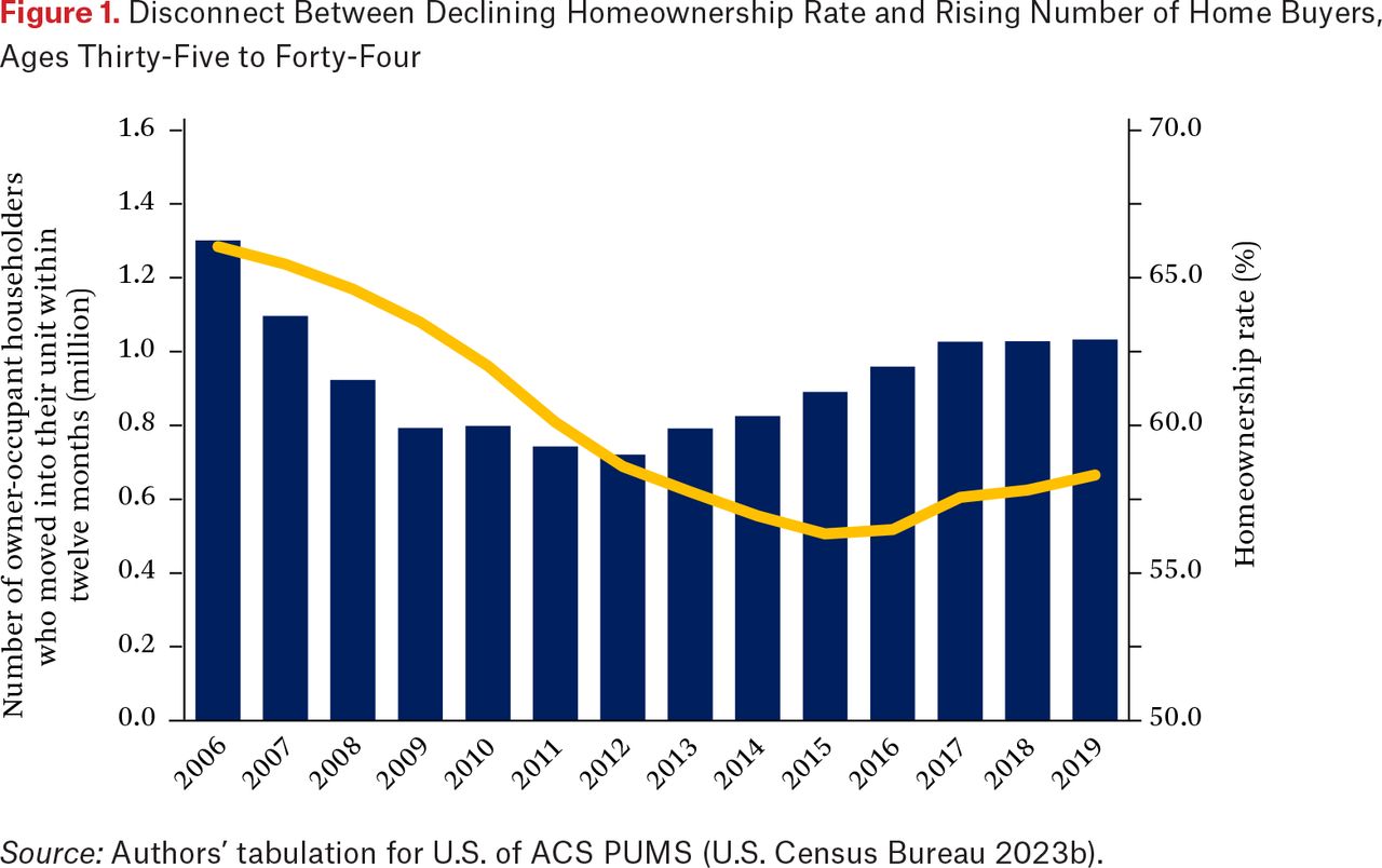
A striking anomaly, discovered by Patrick Simmons at Fannie Mae (Myers, Lee, and Simmons 2020), was that actual homebuying by young adults was rapidly rising even while their homeownership rate drifted downward (figure 1). Explanation for the apparent paradox is that the unrecognized structural lag built into the current homeownership rate caused accumulation histories over several previous years to be carried forward into current trends, with misleading result.6 This pronounced lag risked skewing public perceptions about the health of the housing market and millennials’ desires to buy homes, as discussed later.

Disconnect Between Declining Homeownership Rate and Rising Number of Home Buyers, Ages Thirty-Five to Forty-Four
Source: Authors’ tabulation for U.S. of ACS PUMS (U.S. Census Bureau 2023b).
Age Relationships Can Be Misspecified with Dramatic Error
Economists may have learned to be wary of using age data after witnessing the highly publicized error of Gregory Mankiw and David Weil (1989), who linked age groups to trends in house values. The two scholars observed age differences in housing expenditures in 1980 census data, finding much lower expenditures for age groups after forty-five, which is just where the leading cohort of the baby boom generation (born 1946 to 1964) was positioned in 1990. With these age inputs, their model estimated that house values would fall by 47 percent between 1990 and 2010; instead, the opposite occurred, values doubling. In fact, the boomers had been traveling on higher trajectories of housing consumption all along and should never have been assumed to drop down as they aged to the older, smaller, and less expensive homes of their parents. This paper was criticized for many reasons (Green and Hendershott 1996; Woodward 1994), but it was the simple matter of confusing age groups and cohorts that led their forecast so badly astray (Pitkin and Myers 1994). Our takeaway from this pivotal lesson is that legacy effects embedded in cohorts’ accumulated homeownership rates require that age data should be structured as cohorts that grow older, not confusing this with age differences that are comparisons across cohorts in fixed periods.
Long Swings and Economic Cycles
Aging of cohorts occurs within another time context—namely, the passage of historical time that is marked by economic cycles of expansion and contraction. Macroeconomists in the mid-twentieth century were sensitized to boom-bust cycles in the economy enveloped in longer swings of population and economic growth. The leading proponent, Simon Kuznets (1958) emphasized long swings of rising and falling consumer demand of some fifteen to twenty-five years duration as overlays to short-term business cycles of expansion and contraction. Richard Easterlin (1968) showed specifically how long swings in fertility rates shaped future swings in labor force and economy, and that relative cohort size also dictated degree of competition among peers in age-specific activities, thus influencing relative well-being (Easterlin 1987).
Impacts on housing construction and consumption played a pivotal role. Surging numbers of young adults require housing for newly formed families, which synchronized rising investment in construction and furnishings, and spurred employment expansion. But the great expense of the durable housing good causes greater reliance on financing. Thus the timing of new construction to meet population demands can be delayed by high interest rates, or other adverse circumstances, but delay makes the accumulated demographic pressure stronger. This long cyclical relation of housing to population change was developed in early detail by Burnham Campbell (1966), and recent scholars have confirmed and extended these relationships using contemporary econometric methods (Francke and Korevaar 2022; Monnet and Wolf 2017).
Recent Surprise Reversals After Peak Millennials
Impacts of relative cohort size are slow acting and often overshadowed by dramatic period events such as recessions. Widespread misreading of the burgeoning millennial generation after the 2010 Census took on its own consequences. City leaders and urban experts saw that the young millennial generation was flocking to major cities, reversing the decades-long trend of big-city population decline. The popular narrative for this back-to-the-city shift was one of an epic culture change: young millennials had discovered strong new preferences for urban living. However, systematic review of survey evidence found the primary support for these “new preferences” was simply millennials’ greatly increased urban presence (Myers 2016).
Millennials had always been 32 percent more numerous from the time of their birth in the peak cohort of 1990, rising rapidly from the low numbers of Generation X born annually in the late 1970s. As could be foreseen, the fertility upturn led to a strong upswing twenty to twenty-five years later in districts popular with young singles. This burgeoning pool was amplified further by the Great Recession’s prolonged aftermath of depressed economic and housing opportunities, which stalled the usual career and housing advancement by young adults. Attractions to both urban and suburban living remained strong (Lee 2020), but the “peak millennials” thesis (Myers 2016) held that once this rising wave passed age twenty-five after 2015, and assuming effects of the Great Recession finally abated, the ranks of maturing young people would exercise pent-up demand and move outward in search of larger housing units. In fact, by the end of decade, annual Census Bureau estimates revealed a very strong outward population shift began in large cities in 2015 and accelerated in 2018, well before the added pandemic shock (Frey 2021; Lee 2022). In addition, after 2016, their homeownership rates also shot forward, as will be closely examined.
POPULATION COHORTS AND BIG CHANGES AHEAD
Population aging occurs slowly and steadily, a year at a time, but this can result occasionally in rapid reversals of population impacts at key ages. On the surface, this potential is not always apparent. Robert Shiller received a Nobel prize for his work on volatile asset bubbles, as addressed in both housing and stock markets. Population growth over the last century was featured as one of three trends potentially underlying real house prices in Irrational Exuberance (Shiller 2015). Neither the trends in interest rates, real building costs, or total population appear correlated with extremely volatile home prices after 1995 (see figure A.1 in the online appendix: https://www.rsfjournal.org/content/11/1/86/tab-supplemental), but population was singled out for particular dismissal, noting that “population growth has been steady and gradual” (Shiller 2015, 19) and is otherwise unnotable.7
In contrast to a steady upward line of population growth, population wields its most acute influence through the potential impacts of age waves, which are best explained as long swings in cohort size at birth that then travel across age groups as cohorts grow older. Both upswings and downswings have potential impacts in specific age groups. Revealing these impacts, first, we structure the population data to reveal the age detail of changes over a long-term trend.8 In a following section, we estimate the slowing and accelerating rates of cohorts’ housing consumption during periods of recession or prosperity, but first we describe only what was knowable in advance about the size differences between cohorts and the timing of arrival in particularly sensitive ages.
Oscillating Age Waves
A closer integration of population and housing is built from the ground up by starting with the population data rather than the households already formed. The changing age structure of the U.S. population is initiated by fluctuations in annual births, depressed in the 1920s and 1930s, then booming from the 1940s to early 1960s, and depressed once again through the 1970s, but finally rising again in the 1980s to the peak of the millennial generation born in 1990. The oscillation between falling and then rising sizes of birth cohorts has potential buffeting impacts. These native-born cohorts are augmented by additional residents who are foreign born, typically joining the cohort in their twenties. However, the great bulk of variation in recent decades is due to past fluctuations in native-born births.
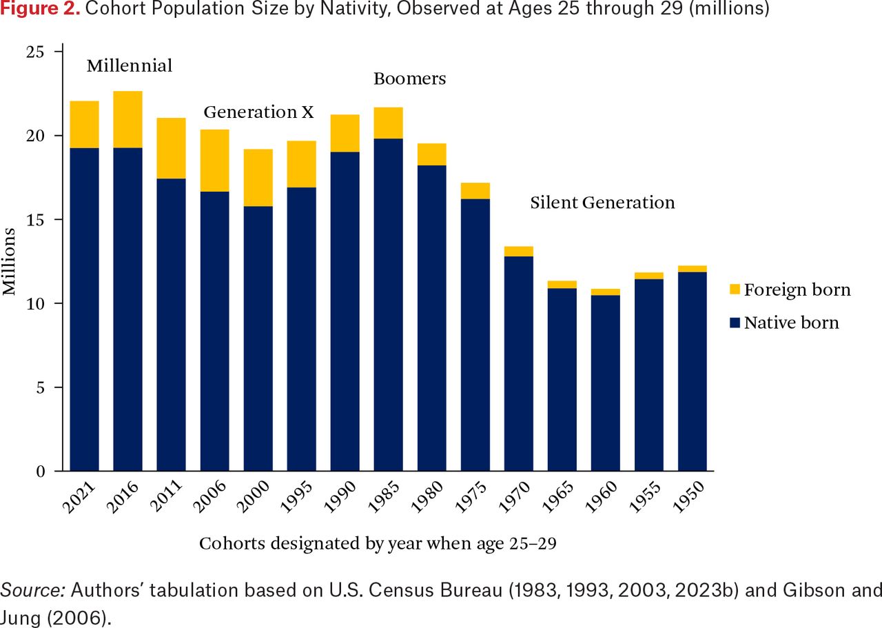
Our first analysis addresses the size of cohorts in different generations, both U.S. born and foreign born, choosing an age that makes most sense for comparison. For this we aim to compare the cohorts when they were age twenty-five to twenty-nine, strongly establishing themselves as young adults. The earliest cohorts observed are members of the silent generation, born from 1925 to 1945, a decade or two earlier than the baby boomers who followed after them.9 These early cohorts were all quite small, and the baby boomers (born 1946 to 1964) arrived in a series of four larger five-year cohorts. The two youngest cohorts among the boomers started to include foreign-born age peers, which figure 2 accounts for as an added layer. The youngest five-year cohort among the boomers began to enter adulthood with smaller size due to fewer U.S.-born births from 1960 to 1964, and then the much smaller Generation X (born 1965 to 1979) made its entrance.

Whether we compare only the U.S.-born cohort members or the population totals with foreign born added, the cohort reaching age twenty-five to twenty-nine in 2000 is the smallest in decades. Adding to the diminishing effect of this cohort, it follows at least one other cohort also with substantially diminished size, the two of which would fill the twenty-five to thirty-four age group, long considered the fount of housing demand, with much smaller numbers. In 2005, these shrunken cohorts advanced to thirty to thirty-nine, depleting the age range most crucial to home buying, as addressed in the next section. This sinking demographic was softening potential demand in the exact period of the housing bubble when, curiously, housing prices soared despite population decline in key age groups for owner-occupancy.
We devote most attention to the volatile period after 2006,10 beginning with the peak of the economic expansion and then deep decline into the Great Recession, whose effects bottomed only in 2011. From that point, a slow recovery proceeded to 2016, then accelerating housing demand to 2021 even amid the pandemic and brief 2020 recession during the COVID shutdown. The population numbers of each cohort are fairly stable across these periods, while the housing behavior to be investigated is highly variable.
In the analysis that follows, initially we select only the U.S.-born adults, because we wish to highlight changes that were knowable for a long time (numbers since birth) but may have been overlooked. Immigration is more variable and is a growing factor in certain years, adding to total housing demand. Immediately apparent in figure 2 is that the expanding immigration of the 1990s was helpful for buffering the downturn in population size of Generation X cohorts, especially in 2000 and 2006. Nonetheless, even with immigrant additions, comparing the boomer cohort age twenty-five to twenty-nine in 1985 with the Generation X cohort following that age in 2000 still shows a decline of 11.5 percent, followed by a renewed rise of 18.5 percent to the peak millennial cohort in 2016. After 2000, immigration growth slowed and virtually no change is observed in the size of the foreign-born component.11 The key point remains that, nationwide and in the great majority of states, the oscillation of the native-born births is the underlying driver of growth between cohorts entering the twenty-five to twenty-nine age group.
Impacts of Cohort Swings on Growth in Key Age Groups
Changes in population size across cohorts is revealed in a sequence of expansion and contraction. Some fifteen years of growth (boomer cohorts) was followed by fifteen years of downswing (last of the boomers, plus Generation X), followed once more by fifteen years of upswing to the peak millennials. The fifteen-year intervals are long enough to exceed a single business cycle and create an impression of ongoing, persistent change in one direction, before those implicit expectations may be undermined by a reversal. The complexity is that these pulses of growth or contraction arrive at different age groups in different historical years, cohorts arriving first in the youngest ages, before advancing to next older ages. Thus, the pivotal reversal in cohort size occurs in successively older ages in successively later time periods, never synchronized for all ages. Far from following Shiller’s steady upward line, population changes by age group are volatile, yet predictable.
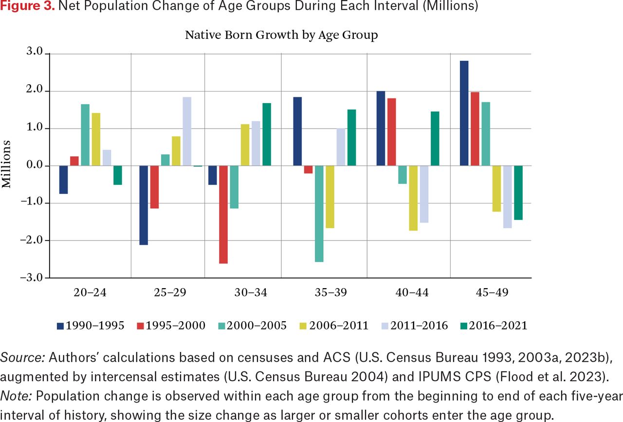
This population swing within each age group is illustrated in figure 3. The oldest age shown, forty-five to forty-nine, contained the last remnants of growth from baby boomers in the 1990s, falling to prolonged losses when smaller Generation X cohorts entered after 2006. The next youngest age group, forty to forty-four, picked up renewed growth beginning after 2016, but the thirty-five to thirty-nine age group was already experiencing that renewal by 2011, and the thirty to thirty-four age group experienced the upswing for fifteen years, beginning after 2006. The comparison of upswing to preceding population losses has strong implications for reversals in both rental and ownership demand in key ages.

Net Population Change of Age Groups During Each Interval (Millions)
Source: Authors’ calculations based on censuses and ACS (U.S. Census Bureau 1993, 2003a, 2023b), augmented by intercensal estimates (U.S. Census Bureau 2004) and IPUMS CPS (Flood et al. 2023).
Note: Population change is observed within each age group from the beginning to end of each five-year interval of history, showing the size change as larger or smaller cohorts enter the age group.
EXPECTED HOUSING DEMAND AND INTERVENING REALITY
The twenty-first-century stage was set for substantial housing growth due to the rising size of prime age groups as the large millennial cohorts reached their high-impact housing age after 2010. However, a major collapse of the housing financial system intervened, spawning the Great Recession. In addition, some critical faults in the data guidance systems were exposed, so that the impending demographic changes were insufficiently connected to policymaking. Housing would still be tethered to population, but with much confusion and unanticipated delay.
Disruption by the Crash and the Regulatory Response
The institutions that foster housing opportunities are crucial for enabling potential demand to be realized. The first two decades of the century were wildly volatile in that regard. In the first decade loose credit and lax regulation were one way the George W. Bush administration could promote their “ownership society,” but Shiller (2015, 60) dryly notes that “this political philosophy did not emphasize the importance of government monitoring of mortgage lending practices.” The lack of regulatory oversight during the housing bubble and foreclosure crisis was very widely criticized after the fact.12 Other parties blamed the burgeoning price escalation and mounting foreclosures on the fair housing initiatives that began under the Bill Clinton (Democratic) administration in the 1990s and may have opened the laissez faire floodgates in the Bush (Republican) administration that followed (Aalbers 2009). Yet Adam Levitin and Susan Wachter (2020, 175) are very clear in their assessment: “The bubble was not the result of government policies supporting fair lending and affordable housing, but rather the result of a shift in mortgage financing from quasi-regulated securitization by the GSE duopoly [that is, Fannie Mae and Freddie Mac] to unregulated securitization by Wall Street.”
Indeed, the thorough postmortem provided in Levitin and Wachter’s (2020) Great American Housing Bubble attributes the price run-up from 2002 to 2006 almost entirely to easy credit that encouraged people to purchase more housing than they could normally afford:
The expansion of mortgage credit collided with an inelastic housing supply, with the result that home prices were bid up. . . . But because the higher home prices depended on mispriced credit and on underwriting that would predictably raise default rates, once the momentum in demand growth and price rises ended, the price increase was unsustainable. In other words, home prices were bid up beyond fundamentals, and when the credit supply then ultimately faltered because of the unsustainable nature of the mortgage products it was financing and the exhaustion of the borrower pool, a collapse in home prices was inevitable. (Levitin and Wachter 2020, 164, emphasis added)
In response to the dire financial crisis that followed the crash of the housing bubble, and the mounting toll of the subprime foreclosure crisis with nearly eight million lost homes, the federal government was motivated to respond with major new restraints on the banking system that would severely tighten a very loose system of credit approvals. Through the Dodd-Frank legislation enacted in 2010 and subsequent agency guidelines (Bailey et al. 2017), the pipeline for home loans was sharply constricted, not only raising the qualifying criteria but also greatly expanding documentation requirements and slowing the processing speed so that many fewer mortgage applications could be approved.13 The justified goal was to correct for the excesses of the loose regulation during the housing bubble and make real estate lending much safer. However, less willingness to take on risk means fewer opportunities for home buyers below the top echelon of income and credit, dropping the homeownership rate 2.3 points lower than it would have been under the stricter, pre-bubble standards prevailing in 2001 (Acolin et al. 2016; Wachter and Acolin 2022). The extreme, overly tight correction is graphically revealed in the Urban Institute’s Housing Credit Availability Index (as shown in figure A.2 in the online appendix).14
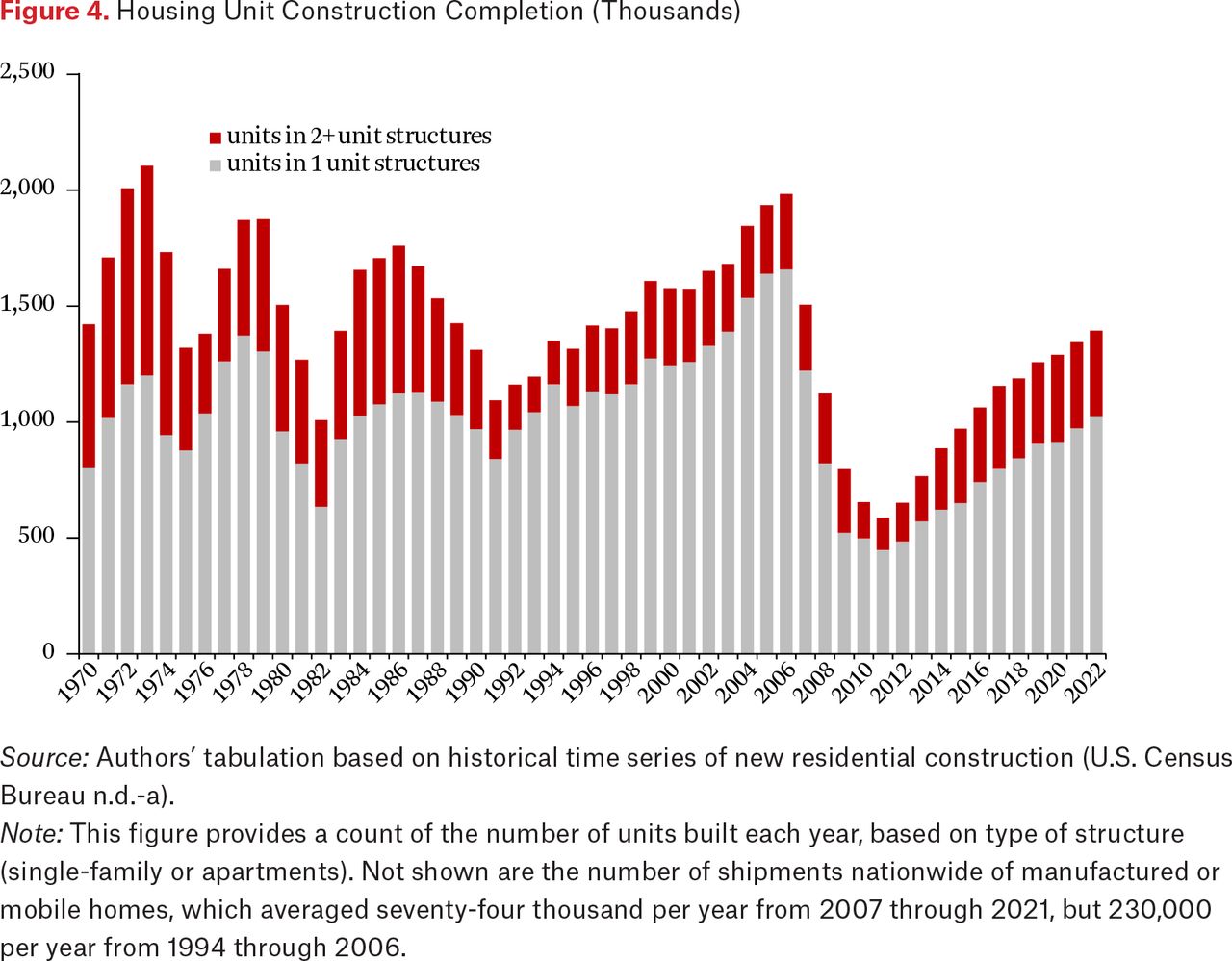
Housing construction also suffered in the decade of the 2010s, facing its own difficulties in assembling financing, as well as labor shortages, NIMBY resistance, and other difficulties in land assembly and permitting approvals (Dietz 2020). All the while, growing demand has pressed against this restricted supply, bidding up prices, and also forcing would-be buyers into rental competition, raising rents and reducing affordability there. The record of pullback in housing construction is stunning (figure 4). It would appear that a spike of two years of overbuilding during the bubble was followed by nine years of construction that barely exceeded one million units per year or much less.

Housing Unit Construction Completion (Thousands)
Source: Authors’ tabulation based on historical time series of new residential construction (U.S. Census Bureau n.d.-a).
Note: This figure provides a count of the number of units built each year, based on type of structure (single-family or apartments). Not shown are the number of shipments nationwide of manufactured or mobile homes, which averaged seventy-four thousand per year from 2007 through 2021, but 230,000 per year from 1994 through 2006.
Confusion over Misleading Signs and Interpretations
All this tightening of lending and construction—designed to guard against excesses of the soft market in the bubble years—seems worse in the face of the oncoming tsunami of millennial housing demand. However, it is not clear that preparing for this coming large generation was ever recognized as a priority. Three factors may have prevented or distracted attention.
Lack of Data Linking Demographics and Mortgages
Foremost was the underlying lack of data linking mortgage finance and demographics. The mortgage databases widely relied upon by analysts in housing finance contained no demographic characteristics about the borrowers. Restricted by the Privacy Act of 1974, neither race or age were systematically recorded, at least until 2014.15 Even though separate databases collected by the Census Bureau do link demographics and homeownership, they do not extend to mortgage characteristics relied on by financial analysts for calculating industry risks of default and foreclosure.16 The lack of householder age in core databases in earlier decades prevented developing trusted models using age with financial data. Moreover, the widely known Mankiw and Weil (1989) debacle discussed earlier may also have discouraged many housing economists from risking further experimentation with the census age data.
Attention Preempted by Emergencies Instead of Long-Term Demographic Trends
A second factor is that both analysts and policy makers were preoccupied by more urgent problems—namely, the long-building foreclosure crisis (Immergluck 2009). An enduring problem is that coming demographic changes, in contrast, were often distant concerns, falling beyond any current term of political office.17 However, in this case, the unrecognized entry of smaller cohorts into prime ages for homebuying softened the market base through Levitin and Wachter’s “exhaustion of the borrower pool.” Ironically, the overlooked demographic change helped collapse prices and may have intensified the wave of foreclosures, thus contributing to the global financial crisis and Great Recession.
Misled by the Lagging Homeownership Rate and Confusion About Millennials
After 2010, much larger young cohorts began to arrive in cities, but the significance of the millennials for housing was uncertain. In the prolonged aftermath of the Great Recession, there was understandable confusion about where the housing market was headed and what policy changes could alter that (Weisman 2015). The most persuasive explanations made key indicators the center of shared understandings, an example of Shiller’s (2019) depiction of viral “narrative economics” as a coordinating feature in markets. Accompanying the narrative of new preferences for millennials and urban revival, as described earlier, which misled about the persistence of urban residence preferences displayed during the recession, a reinforcing narrative emerged of abandoned homeownership preference based on foreclosures and falling homeownership rates. The foreclosure crisis certainly could be read as a general warning of the dangers of promoting homeownership, but the deep decline in homeownership rates from their peak in 2005 and continuing twelve years was especially alarming. The negative role of constricted access to mortgage credit was clear to experts in housing finance (Acolin et al. 2016; Urban Institute 2023), but access remained little improved for a decade or more (figure A.2).
Instead, broad attention fixated on key evidence in support of the abandoned homeownership narrative—namely, a graphic display of the homeownership trend that was issued in identical format every three months in periodic news releases for the Census Bureau’s homeownership and housing vacancies report (figure 5). These data have vital importance, given their description as “used extensively by public and private sector organizations to evaluate the need for new housing programs and initiatives” (U.S. Census Bureau, n.d.-c). In fact, Shiller (2019, 45, 97) emphasized how such a regularly repeated data indicator and graphic can focus attention through repetition and drum home a popular narrative explaining a trend. In this case, the graphic downturn in homeownership was dramatized by the fresh release of each quarterly report’s extension of homeownership decline, initially dropping only 2 percentage points from the peak homeownership rate of 69 percent in 2005 and 2006 (U.S. Census Bureau 2016, table 4) through the recession ending by 2010, but then extending after the recession at even-faster pace of decline, dropping 4 more percentage points over the next six years (finally ceasing in 2016). The decline also was visibly magnified by the graphic’s use of a y-axis truncated to a range of only 62 to 70 percent. This long, increasing drumbeat of decline, revealed three months at a time, negatively influenced all parties—builders, lenders, consumers, and policymakers, as well as opinion leaders among columnists—about the wisdom of planning for more homeownership. Because the graphic display was unaccompanied by any explanatory text about the lagged nature of ownership rates, or any current evidence of rising home buying (see figure 1), until 2017 the impact seemed to foster fear of bottomless decline.

Homeownership Trend in Quarterly Press Release Through 2016
Source: U.S. Census Bureau 2016, figure 4.
Note: This figure, example taken from 2016, is a standard part of the press release for the Housing Vacancies and Homeownership report. The figure was repeated quarterly in identical format from 2010 through 2023 (updated three months each time).
POPULATION-BASED ESTIMATES OF HOUSING DEMAND
In hindsight, and outside these major disruptions, how much housing demand for rentals and owned homes was reasonable to have expected and is now unmet? Our empirical task here is measuring the changes in occupancy status over a succession of five-year intervals, and then comparing that to what might have been expected if conditions of 2000 had continued.
Comparisons of population and housing rely on one of the most basic units of housing demand, which is the number of occupied housing units. The long-established method of headship (or householder) rates is used to convert between population and number of occupied housing units.18 The tradition in housing research is to first form households as a percentage of population and then form owner and renter occupancies as a share of those households. However, a growing alternative practice is to treat rental and owner occupancies directly as a percentage of the underlying population, that is, per capita not per household, so that the household formation is partitioned into two components summing to total household formations. Householders per capita in an age group equals renters plus owners per capita in the same age group.19 We aim to describe these outcomes specific to age groups (or racial groups) and specific to the different periods used to describe the population cohorts.
This identity relation of household formation represents actual demand only to the extent that there is sufficient housing supply to accommodate all of the would-be households. The crucial assumption is that an efficient supply response will produce enough units to accommodate the expected preferences for occupancy. However, the record of constricted housing construction after the Great Recession has not been favorable for accommodating (and revealing) the full housing demand among either renters or owners. As shown in figure 4, the downturn in construction beginning in 2007 fell to deeper levels than any time in the last sixty years, falling below one million completions for the first time and remaining below that level several years. A key result was that for at least eight years in the recent decade, newly built units failed to exceed the growth in household occupancies (Joint Center for Housing Studies 2019), providing no increase in vacancies, which Jonathan Spader (2022) finds approached an historical low.20
Owner and Renter Occupancies by Age Before and After the Crash
In analysis to follow, we closely track the observed rates of owner and renter household formations, arranging these in alternative configurations to reveal particular insights. Of particular interest is how greatly the owner and renter formations after 2006 differ from those in the 1990s or bubble of the early 2000s. The changes are concentrated in particular age ranges, reflecting a decade-long recovery after the crash and eventually a sharp upswing.
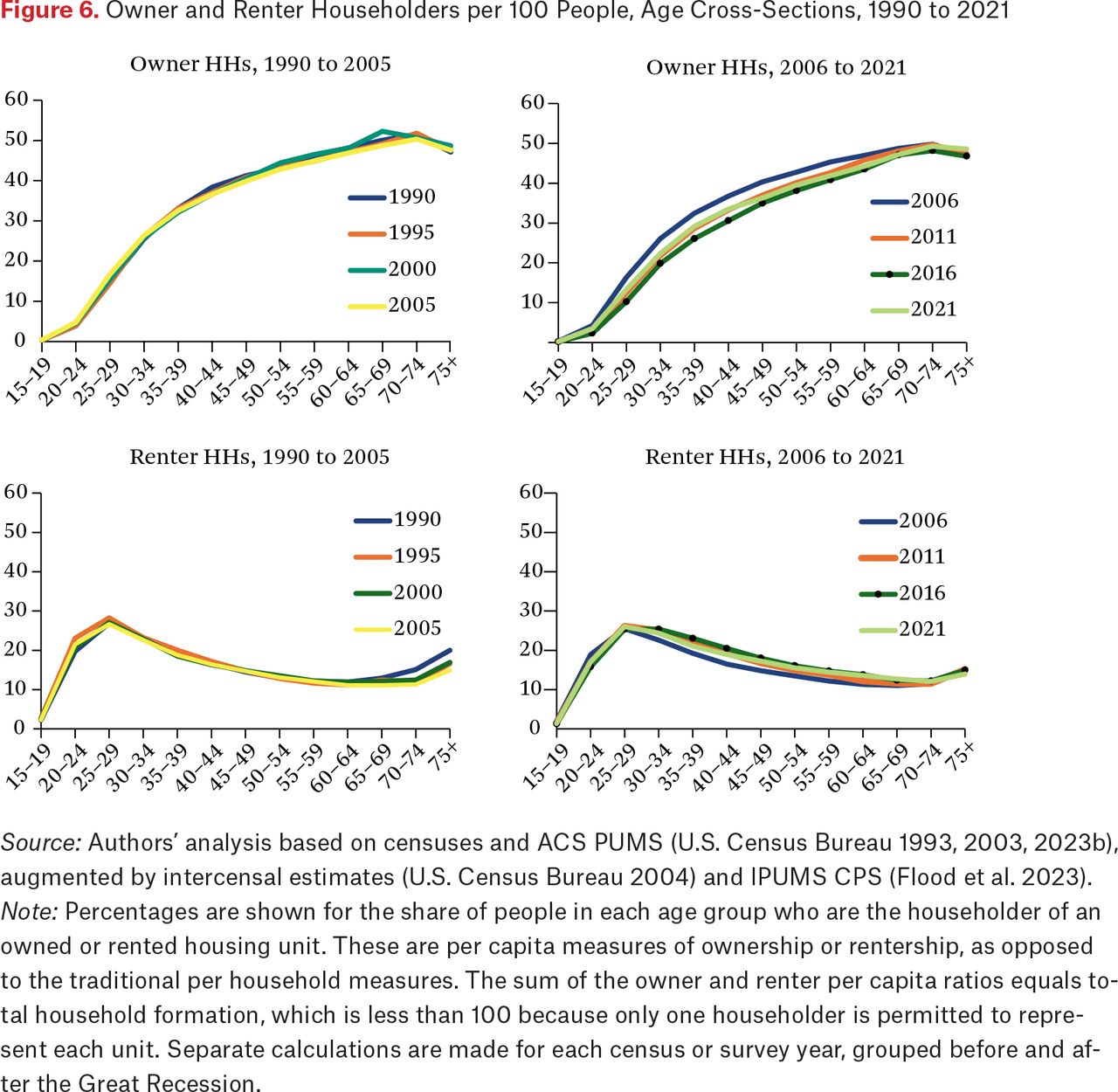
The age cross-sectional probabilities of owning and renting are observed separately in each census year or survey year, the two upper plots showing per capita homeownership, the bottom plots per capita renters (figure 6). Earlier points in time are grouped in the left-side plots for 1990 through 2005; the right side covers 2006 to 2021. We see a very close similarity of housing occupancy in survey years before the Great Recession (figure 6, left side). Within both owners and renters, the lines are virtually on top of each other. The overall pattern is a rise of homeownership up to age seventy, but among renters a rapid burst of rental formation during their twenties that then declines until it rises slightly in their later years.

Owner and Renter Householders per 100 People, Age Cross-Sections, 1990 to 2021
Source: Authors’ analysis based on censuses and ACS PUMS (U.S. Census Bureau 1993, 2003, 2023b), augmented by intercensal estimates (U.S. Census Bureau 2004) and IPUMS CPS (Flood et al. 2023).
Note: Percentages are shown for the share of people in each age group who are the householder of an owned or rented housing unit. These are per capita measures of ownership or rentership, as opposed to the traditional per household measures. The sum of the owner and renter per capita ratios equals total household formation, which is less than 100 because only one householder is permitted to represent each unit. Separate calculations are made for each census or survey year, grouped before and after the Great Recession.
This steady consistency of household occupancies broke down after 2006, with the crash of the housing bubble and plunge into the Great Recession. Thereafter, age cross-sectional plots among both renters and owners became much more differentiated across the time periods (figure 6, right side). Viewing the owner occupancies, probabilities by age were highest in 2006, falling to 2011 in the trough of the recession losses,21 and then falling still further to 2016 (line marked with black dots), when the nation’s aggregate ownership rate reached its lowest point. Thereafter, a rebound proceeded to 2021, which is very close to the level of 2011 in most age groups.
It might seem self-evident that a loss in the homeownership rate implies a gain in rentership, and most of the lost homeowners over this period likely were diverted into renting (Myers et al. 2016). However, the rental plot is not symmetrical, that is, with rental increases matching homeowner decreases.22 The diversion of owners into rentals created greater rental competition, with rents escalating far more than incomes, as noted earlier. Some portion of the expected, would-be renters were dislodged from independent quarters and doubled up with roommates or family members. Overall, the result was lowered household formation.
Active Demand by Cohorts Progressing into Rented or Owned Units
The term household formation may be misleading, because formation connotes an act of recent household status achievement. In fact, most adults are engaged in maintaining previously attained household status, especially when they are middle age and older. As seen in table 1, 73.5 percent of owners older than fifty-five have lived more than ten years in their current housing unit, as have 33.1 percent of renters. Thus their current rates of renter or owner occupancy do not reflect a formation or recent activity in the housing market.
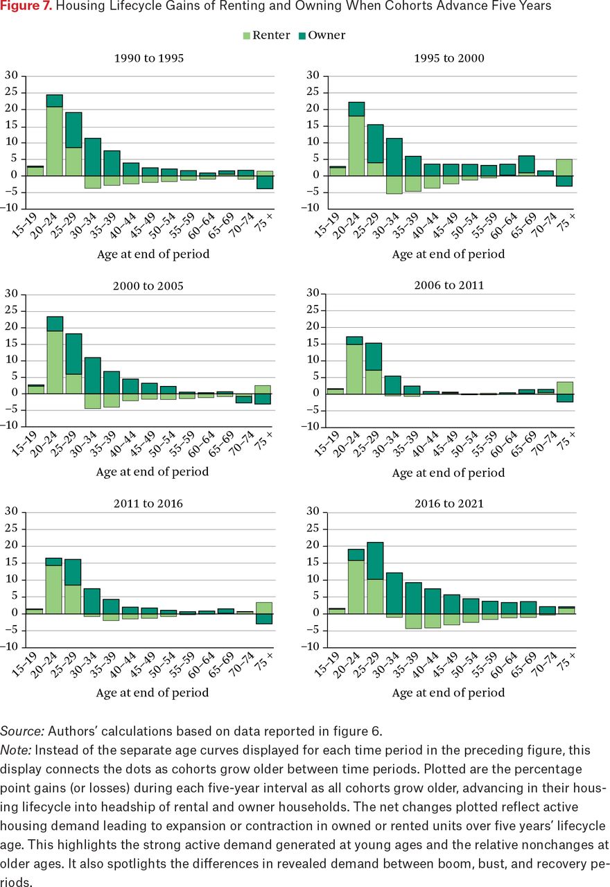
A better method is needed for estimating and visualizing the housing demand newly expressed in a period. Here we propose to estimate net increases in cohorts’ housing occupancies as they newly advance to the next age between periods.23 Our cohort housing lifecycle method highlights the incremental changes in five-year intervals. A total of six periods are separately estimated, composed of two half-decades in the 1990s, two in the 2000s, and two more in the 2010s.24 We expect to find a sharp downturn in active household formation during the recession interval of 2006 to 2011, followed by a recovery from 2011 to 2016 and extended further in 2016 to 2021. Cohorts passing through young adult age groups are likely to make very rapid advances in demand, settling down thereafter. What is not known is how different were the cohort advances in different time periods of boom, bust, or recovery. The six time intervals each could foster a unique lifecycle of housing increases, revealing active demand distinct to each time period. Facilitating comparison, figure 7 affords a visual array of net cohort changes for both owners and renters, within each age group, and across the six intervals. As one example, the cohort arriving at age thirty to thirty-four in 1995 added 12 percentage points to the cohort’s accumulated ownership rate per capita since the beginning of the five-year period in 1990. In the same interval, rental occupancy per capita declined by 3 percentage points, yielding a total additional household formation of 9 percent of the cohort population.

Housing Lifecycle Gains of Renting and Owning When Cohorts Advance Five Years
Source: Authors’ calculations based on data reported in figure 6.
Note: Instead of the separate age curves displayed for each time period in the preceding figure, this display connects the dots as cohorts grow older between time periods. Plotted are the percentage point gains (or losses) during each five-year interval as all cohorts grow older, advancing in their housing lifecycle into headship of rental and owner households. The net changes plotted reflect active housing demand leading to expansion or contraction in owned or rented units over five years’ lifecycle age. This highlights the strong active demand generated at young ages and the relative nonchanges at older ages. It also spotlights the differences in revealed demand between boom, bust, and recovery periods.
The compiled housing lifecycle follows the same general pattern in all periods: net household formations are dominated by people under age forty, renting begins to decline after age thirty, and homeownership rises rapidly through forty but continues to climb slowly. A small but continuous stream of net ownership gains occurs among middle-aged and elderly people, less so in times of recession and early recovery. It is not surprising how similar the three intervals preceding the 2006 mid-decade peak of the housing bubble were, which is consistent with the close similarity found among the age cross-sections pre-recession.
The next two intervals, beginning in 2006 and 2011, correspond to ten years of discouragement about housing in America, first in the Great Recession and then in its lingering impacts of depressed ownership rates. Unlike in earlier periods, virtually no net changes occurred after age forty other than adjustments late in life at age seventy-five or older. Cohort progress was virtually flat for ten years, showing no net housing changes. Yet even in those bleak times, it is remarkable how robust the household formation of people under age thirty was. Growing into young adulthood prompts rapid increase in housing needs as partnerships bond and families grow. Even during the recession interval between 2006 and 2011, sizable shares of people ages twenty to twenty-nine became householders, especially as renters and, despite the depths of the economic recession, this expansion of housing occupancy by cohorts was only about one-quarter less than the norm in the late 1990s (figure 7).
More striking in the interval of 2006 to 2011 was the absence of gains in early middle-aged homeownership between the ages of thirty and fifty-four, contrasting with the previous substantial gains seen from 2000 to 2005 and in the late 1990s. Cohorts traversing this age range instead held on to their rentals, whereas before they vacated rentals while transitioning into homeownership. Reflecting the prolonged effects of the Great Recession, virtually the same pattern was sustained five years later during the protracted recovery from 2011 to 2016. Only a slight net outflow from renting and a slightly larger increase in owning occurred after age thirty-four.
POST-2016 RECOVERY OF PENT-UP DEMAND
After a decade of frustrated housing attainments, the abrupt and forceful revival of housing demand might seem a mirage. How much of the depressed formations was deferred as pent-up demand and how much of the shortfall was actually recovered? We wonder also how equally was this new progress shared among all age and racial groups?
Rebound of Cohort Progress from 2016 to 2021
The revival of lifecycle progress after 2016 was extraordinary. Evidence was clear that homeownership rates began to rise in 2017, encouraged by a continuing rise in incomes and also motivated by several years of rising house prices that raised expectations for future gains.25 In the rebound from 2016 to 2021, as new construction of multifamily units also began to reach higher volumes, we see a large gain in new household formations among ages twenty to twenty-nine similar to what prevailed before the Great Recession, though this is slightly delayed to age twenty-five to twenty-nine relative to twenty to twenty-four, and still skewed more to rentals at this age than in intervals pre-2006 (figure 7). However, above age thirty, the substantial outflow from renting resumed as before when more households transitioned to owning. Especially noteworthy after 2016 are the unprecedented strong gains in added homeowners from ages thirty-five through sixty-nine. We strongly suspect this must be a middle-age catch-up for a decade’s pent-up housing demand incurred during the restraints from 2006 to 2016.
Pent-up demand is often a speculative judgment, but evidence here shows that, relative to pre-2006 norms, the foregone achievements of two consecutive periods (2006 to 2011 and 2011 to 2016) were at least partially fulfilled by the end of the decade, when cohorts advanced at accelerated rates in later age groups. Thus, we could explain the rising ownership in older age groups as largely due to postponed demand carried forward within cohorts.26 These late arrivals were surely benefited by the lowering of interest rates late in the decade and to 2021. The late arrivals in homeownership might also be marginal buyers whose incomes are more limited, dependent on pooling multiple incomes in the household, including drawing on earnings of grown children. In contrast, at the young end of the housing lifecycle is now broad awareness of the role of privileged family assistance in helping young adults to purchase homes many years earlier than if they had to save their own downpayments (Bhutta et al. 2020; Lee et al. 2020).
How Close Is the New Accumulated Status to Normal?
What have been the net changes for owners and renters in the first two decades of this century, after taking account of the setbacks around the Great Recession and then the major catch-up in the last five years? And how have the major race and ethnic groups fared during this period of prolonged recession and recovery? How close to normal is 2021?
Disproportionate and Undermeasured Impacts on Renters
As of 2021, the Census Bureau estimates the total number of U.S. households as 127.55 million, 83.49 million owners and 44.06 million renters.27 These totals differ substantially from what would have been expected had the population by age and race group grown as observed over the two decades but the per capita rates of owner and renter household formation by age and race group had maintained their 2000 values (the “expected”). The gap between the observed and expected household totals among owners grew to be 5.04 million short of what would be expected for 2011, at the bottom of the recession, but virtually no difference was found in number of renters expected. The shortfall among owners continued to deepen through 2016, reaching 8.61 million by 2016, but new construction was still lagging and population in the key age range for formations was growing.
In what might seem a paradox, renters bore the brunt of the homeownership declines that continued from 2011 to 2016. Even though the losses appear attributed all to owners and none among renters, in fact, spillovers of would-be homeowners swamped the rental market through a cascade of diverted demand that displaced a nearly equivalent number of previously expected renters (Myers et al. 2016). The excess of unexpected renters rose only to 0.64 million by 2016. Because so few “extra” renters did not begin to balance the shortfall of owners, total household formation through 2016 was reduced by 7.96 million. The lost households are not directly observable but likely constitute the most vulnerable renters that did not survive competition with the large number of diverted, would-be homeowners added to the rental housing market.
Large Differences in Recovery Between Ethnoracial Groups
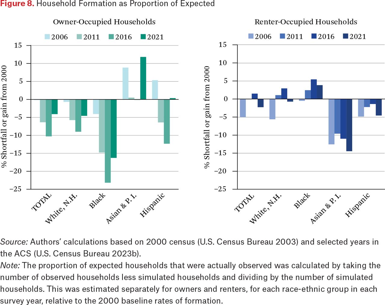
Not all ethnoracial groups fared equally in this housing competition, and not all benefited equally from the eventual recovery. Figure 8 summarizes how each group fared over successive time intervals. For ease of comparing different size groups, shortfalls of owner and renter-occupied households within each ethnoracial group are measured as a proportion of what was expected for each group had 2000 formation rates been maintained. We measure the depths of the shortfall when it was greatest in 2016 and the recovery as of 2021. As reported in table A.1 in the online appendix, accounting for the simulated figures, the number of owners in the total population fell 10.3 percent below expected but recovered to 4.1 percent below expected. Among Whites, specifically, ownership shortfall was 9.0 percent below expected in 2016 but recovered to only 4.6 percent less. However, among Blacks, shortfall was 23.2 percent less than expected but recovered only weakly to 16.3 percent below expected. Experience was very different among the Asian and Pacific Islander group. Ownership held steady in 2011 and 2016 and then improved with a large surplus fully 11.8 percent above expected. Among Hispanics, shortfall was substantial in 2016 (12.3 percent) and then recovered to a slight surplus 0.4 percent.

Household Formation as Proportion of Expected
Source: Authors’ calculations based on 2000 census (U.S. Census Bureau 2003) and selected years in the ACS (U.S. Census Bureau 2023b).
Note: The proportion of expected households that were actually observed was calculated by taking the number of observed households less simulated households and dividing by the number of simulated households. This was estimated separately for owners and renters, for each race-ethnic group in each survey year, relative to the 2000 baseline rates of formation.
Overall, recovery of housing achievements from setbacks of the Great Recession has been very unequal across race and ethnic groups. We find that the Black population recovered only about 30 percent of their steep homeowner losses accrued by 2016, whereas the White population recovered about 49 percent. Hispanics recovered virtually all their losses in homeownership but still had a 4.6 percent reduction among renters; Asian and Pacific Islanders came out 10 percent better in 2021 than in 2000. Unlike all other groups, Blacks not only achieved less of a homeowner recovery than other groups but also continued to sustain a greater number of rental households in 2021 than previously expected.
CONCLUSION
The misalignment of housing and population trends has proven damaging in the twenty-first century, first contributing to the housing bubble, the resulting financial crisis and Great Recession, and later driving acute housing shortages and extreme affordability problems. The first contribution of this article is to revisit the lessons from Kuznets and Easterlin a half century ago about the impacts of long swings in cohort size. We should have seen the millennials coming and formed suitable housing policy in advance. A second contribution is highlighting the long temporal lags of housing occupancies, with homes of older residents selected decades earlier. Active housing change is more common among young adults, but even the homeownership rates of young adults are lagged measurements, reflecting accumulations over preceding years more than the present day.
In particular, third, this lagged accumulation of homeownership rates may have misled about continuing preferences for homeownership. Building on earlier work (Myers, Lee, and Simmons 2020), we demonstrate how the graphic reporting of the nation’s downward trend in homeownership rates effectively synchronized misperceptions of continued downward interest in homebuying, a clear example of Shiller’s (2019) narrative economics persuading minds with simple messages. The resulting unanimity of pessimistic perception among policymakers, lenders, and industry leaders, along with the blind eye to cohort size effects, surely helped delay timely institutional response that could have expedited supply to meet rising potential demand after the Great Recession.
How best could rising demand and its frustration be estimated? A fault of standard homeownership rates is that they are lagged accumulations that overemphasize accomplishments of the past or mislead about recent preference. A fourth contribution of the study therefore is development of the cohort housing lifecycle depiction of active demand, representing recent net changes in owning and renting by cohorts arriving at each age, replicating this for discrete time periods before and after the recession. This method closely marries population and housing by joining the cohort structure of population size and per capita householder behavior rates. Ten years of delayed housing acquisitions between 2006 and 2016 are found to rebound sharply after 2016, albeit incompletely and especially to the detriment of Black households.
Overall, this study describes the destructive interaction of colliding temporal forces of housing, population, and economy. Whether that was due to simple misfortune, overreaction, or lack of supervisory foresight, the result is the greatest misalignment likely ever witnessed in housing or population. The smallest cohorts of young adults in thirty years were allowed to create the greatest housing bubble fueled by easy credit, but the remedies for that—after the fact—tightened the credit for buyers and home builders, aimed at curbing the excesses of the bubble years. Unfortunately, that severe tightening was just in time to welcome the largest cohorts in thirty years, the millennials, with the lowest construction in sixty years and the highest-ever housing cost burdens on young Americans. Clearly, much closer connection of population and housing analysis, tracking the duo together, would seem to be imperative.
FOOTNOTES
↵1. The largest and most comprehensive is the annual American Community Survey, the longest-running the monthly Current Population Survey (including also a derivative quarterly Housing and Vacancy Survey), or the housing focused, biannual American Housing Survey.
↵2. Cohorts have been termed the ideal aggregation for this reason (Ryder 1965). Unlike panel data, cohorts do not follow individuals over time, but all the members of the cohort have experienced key historical events when they were the same age, entering the labor force or the housing market under conditions of recession or prosperity. This holds essential advantage for research in the tumultuous years surrounding the Great Recession (for a discussion, see Myers, Lee, and Simmons 2020).
↵3. The median household income, value, and gross rent in the 1980 Census were $16,841, $47,300, and $243, respectively, in 1979 dollars (U.S. Census Bureau 1983). They were $74,755, $320,900, and $1,300 in the 2022 ACS one-year estimates (U.S. Census Bureau 2023. The dollars terms were adjusted with the Consumer Price Index for All Urban Consumers (CPI-U).
↵4. Temporal variables include survey year, age and cohort, age of housing and year built or vintage, duration of occupancy or year housing was occupied, and (for foreign born) year of immigration.
↵5. The ownership rate of the thirty-five to forty-four age group fell nearly 10 percentage points, from 66.1 to 56.5 percent of households.
↵6. The accumulated ownership rate initially was carried forward from the housing bubble years preceding the recession. Viewed in 2008 and 2010, during the actual recession, the accumulated rate was beginning to decline but still heavily weighted by the high homebuying of the preceding bubble years. By 2012 and 2014, after economic and housing recovery had begun, the ownership rate kept declining because it then embodied more heavily the very low home buying of the preceding recession years. Finally, after 2016 the accumulated rate began rising, given that more years of economic recovery had interceded, but that was not until four years after actual home buying had been on the upswing.
↵7. Shiller (2015) stresses how unimportant is the steady upward line of population growth in his figure 3.1, which is the centerpiece for his housing market discussion, but he never looks beneath the surface of total population. In one of the rare moments when Shiller does touch on demographics, he dismisses the effect of the baby boom generation in reference to the stock market (45–47), not discussing its role in the housing market where demographic linkages to housing are far more motivating.
↵8. We have assembled a database of observations every five years, with population numbers arrayed in five-year age groups, and with matrices repeated separately by race and Hispanic origin. Data are constructed from the censuses of 1990 and 2000, intercensal population estimates by the Census Bureau, and with observations selected from the American Community Survey beginning in 2006, 2011, 2016, and 2021. The CPS/ASEC microdata was used also for the 1995 housing estimates. These population numbers are independently observed in repeated survey years and arrayed in a matrix of age (in rows) by year (period, in columns). In this usual configuration, cohorts effectively travel on the diagonal, growing five years older as they advance across periods.
↵9. We follow the definitions of generations in a recent comprehensive guide (Twenge 2023):
silent generation (born 1925 to 1945)
baby boomers (born 1946 to 1964)
Generation X (born 1965 to 1979)
millennials (born 1980 to 1994)
Generation Z (born 1995 to 2012)
↵10. The first year when complete population and housing data is available in the American Community Survey, our main source for subsequent analysis, is 2006.
↵11. Of course, the immigrant population is much less evenly spread across the nation than the U.S.-born population of boomers, Generation Xers, and millennials. The foreign-born population in a few large metropolitan areas (such as New York, Los Angeles, and Miami) can account for between 30 and 40 percent of total population, compared to 14 percent in the nation, and so the downturn in cohort size is potentially much less steep in those areas.
↵12. In his monetary and fiscal history Alan Blinder (2022, 249, 266) labeled the practices “disgracefully lax,” “outrageous,” and even “went crazy.”
↵13. A CNBC report by Diana Olick in 2015 stressed the extreme increase in paperwork attached to loan applications. The Mortgage Bankers Association determined that the average large bank underwriter who could process 165 loans per month at the peak of the bubble could only complete about thirty-three in 2015.
↵14. In the opinion of the Urban Institute index managers, “Significant space remains to safely expand the credit box. If the current default risk was doubled across all channels, risk would still be well within the pre-crisis standard of 12.5 percent from 2001 to 2003 for the whole mortgage market” (Urban Institute 2023).
↵15. CoreLogic supports the key private sector database on mortgages, lacking demographic characteristics. However, under the Home Mortgage Disclosure Act (1975) the federal government sponsors data collection and reporting that links race and mortgage information. Under a new rule in 2015, the HMDA data added expanded demographic information, featuring age, available only beginning in 2018. Public use datasets collected from Fannie Mae and Freddie Mac by the Federal Housing Finance Agency (FHFA) also omitted age of borrowers. However, a new National Mortgage Database project initiated in 2014 by the FHFA proposed to use existing credit bureau data to assemble a one in twenty representative sample of mortgage borrowers that was authorized to collect age, race, and other household demographic characteristics (Watt 2014).
↵16. Principal are decennial censuses (since 1920 or before), the Housing Vacancy and Homeownership Survey (CPS), including homeownership by age (quarterly since 1965) and the American Community Survey (annual since 2005).
↵17. A telling anecdote related by Alan Blinder in his fiscal and monetary history is that the future retirement of the large baby boom generation “was basically ignored by Bush and his administration’s fiscal policy makers,” finding that “the burgeoning deficits of 2000-2007 were ill-timed [because] the leading edge of the populous baby boom generation would start turning sixty-five late in 2010, making huge demands on both Medicare and Social Security. Nothing was more predictable than that: you just had to add 65 to 1945 to get 2010” (Blinder 2022, 238, emphasis added).
↵18. Only one person in a unit can be designated householder. Even when married couples share a housing unit, the Census Bureau asks the respondents to choose one person to designate as the reference person (the householder) and they are requested to be one of the people whose name is on the rental lease, mortgage, or deed.
↵19. Although the convention is to calculate homeownership rates as the percentage of households that are homeowners, that tradition has been faulted for treating household formation as a separate step that precedes the tenure choice of households (Haurin and Rosenthal 2007; Yu and Myers 2010). In practice, this can produce biased interpretations of the trend in homeownership if the household denominator is expanding or shrinking in unobserved ways, or if different ethnic groups follow different traditions of household formation. Housing demand is also more transparent when the sum of owners per capita and renters per capita equals total household formation.
↵20. A more telling indicator of shortage is simply that rapid increases in rents and house prices also suggested shortage conditions were plaguing the housing market more than a decade after the recession ended. Thus, it does not appear the increase in construction was sufficient to accommodate pent-up demand from earlier in the decade. This strongly suggests that the decade’s household formation may have been suppressed below the number expected to accommodate potential demand (Mathews-Hunter 2021).
↵21. Whereas deep employment losses occurred in 2009, on many indicators the negative effects grew later. The U.S. unemployment rate peaked in 2010, poverty rate peaked in 2011, and real median household income bottomed in 2011 (Myers and Park 2020). On housing measures, house values bottomed in 2011, rents in 2012, and incidence of excess rent burden (30 or 50 percent of income) was highest in 2011. Meanwhile, the homeownership rate declined through 2016.
↵22. For example, the total household formation per capita at age thirty-five to thirty-nine, summing the owners and renters, declined moderately over the entire period between 2006 and 2021 (–1.53 percent of the age group), with nearly twice the decrease accounted by falling ownership (–3.35) as offset by rising rentership (1.82). On balance, household formation in this age group was reduced by 1.53 percentage points.
↵23. Simple age differences include not only the effect of age but also differences between cohorts. Accordingly, pure age effects marking the housing lifecycle can be extracted only by following cohorts as they age. Very different housing experiences are likely in time intervals preceding and following the Great Recession.
↵24. The latter are shifted one year later to account for the 2021 “end of decade” required by data disruptions in the 2020 ACS during the onset of the pandemic. This has the added advantage of beginning the decade in 2011 at the low point of housing and economic impacts from the Great Recession. In turn, that is preceded five years earlier by the 2006 peak of the last housing and economic cycle prior to the recession. The first half of that decade is then represented by 2000 to 2005, which constitutes the boom and bubble period. We find that 2005 and 2006 can equally represent the peak, while each maintains the preferred five-year spacing with preceding or following observations.
↵25. The common user cost model housing economists use to explain homeownership tenure choice, based on prices, rents, and mortgage rates, also includes as its last component “expected price appreciation,” which often can dominate (Himmelberg, Mayer, and Sinai 2005). As Karl Case and Shiller (2003) found, average homebuyers carry very high annual figures in their heads for expected appreciation (averaging 10 percent per year), which is roughly three times what might be the actual long-run average. Once prices started rising under the millennial competition for restricted opportunities and pent-up demand by others, this “expected appreciation” factor made the estimated cost of ownership look ever more attractive.
↵26. Taking one example cohort in figure 7, arriving at age thirty-five to thirty-nine in 2011, instead of the 7-percentage point ownership gain expected over five years in this age span (under the pre-2006 norm), only 2.5 points were achieved during the 2006 to 2011 period, leaving 4.5 points deferred to the next interval from 2011 to 2016. Instead, that also was 1.5 points lower than the expected gain under pre-2006 norms, which now cumulated to 6 points deferred by the cohort when it arrived at its next age (forty-five to forty-nine) in the 2016 to 2021 span. The eventual gain in ownership at that age, 6 points, seems large but was only 3 points greater than the pre-2006 norm expected for increase (3 points) at that age. Thus, the extra 3-point increase observed might be explained as partial catch-up of the 6-point deferred demand accumulated during younger ages and carried forward by the cohort.
↵27. All figures in this section are retrieved from the Census Bureau PUMS files collected in the ACS (U.S. Census Bureau 2023b).
- © 2025 Russell Sage Foundation. Myers, Dowell, Hyojung Lee, and JungHo Park. 2025. “Misalignment of Housing Growth and Population Trends: Cohort Size and Lagging Measurements Through Recession and Recovery.” RSF: The Russell Sage Foundation Journal of the Social Sciences 11(1): 86–109. https://doi.org/10.7758/RSF.2025.11.1.05. Direct correspondence to: Dowell Myers, at dowell{at}usc.edu, Sol Price School of Public Policy, University of Southern California, 650 Childs Way, Los Angeles, CA 90089-0626, United States; Hyojung Lee, at hyojung.lee{at}snu.ac.kr; JungHo Park, at jhpark.planner{at}khu.ac.kr.
Open Access Policy: RSF: The Russell Sage Foundation Journal of the Social Sciences is an open access journal. This article is published under a Creative Commons Attribution-NonCommercial-NoDerivs 3.0 Unported License.
REFERENCES
In this issue


Jump to section
Related Articles
Cited By...
- No citing articles found.