
Abstract
Estimating the lifetime wealth consequences of homeownership is complicated by ongoing events, such as divorce or inheritance, that may shape both homeownership decisions and later-life wealth. We argue that prior research that has not accounted for these dynamic selection processes has overstated the causal effect of homeownership on wealth. Using NLSY79 data and marginal structural models, we find that each additional year of homeownership increases midlife wealth in 2008 by about $6,800, more than 25 percent less than estimates from models that do not account for dynamic selection. Hispanic and African American wealth benefits from each homeownership year are 62 percent and 48 percent as large as those of whites, respectively. Homeownership remains wealth-enhancing in 2012, but shows smaller returns. Our results confirm homeownership’s role in wealth accumulation and that variation in both homeownership rates and the wealth benefits of homeownership contribute to racial and ethnic disparities in midlife wealth holdings.
In the United States, net worth is highly unequally distributed (Keister and Moller 2000), showing strong persistence across generations (Charles and Hurst 2003; Pfeffer and Killewald 2015) and massive racial disparities (Kochhar, Fry, and Taylor 2011; Oliver and Shapiro 2006). Wealth disparities are consequential because wealth facilitates a variety of life chances, including marriage entry and stability (Eads and Tach, this issue; Schneider 2011) and children’s educational and labor market outcomes (Conley 1999, 2001; Orr 2003).
Homeownership is hypothesized to be a key mechanism for wealth accumulation and therefore for the construction and reproduction of asset inequalities. Estimating the contribution of homeownership to wealth at midlife, however, poses substantial methodological and conceptual challenges because wealth is itself a determinant of transitions to homeownership (Di and Liu 2007). The positive association between homeownership and wealth, therefore, may merely reflect that wealthier individuals are more likely to purchase (and keep) homes. Thus, conventional regression models that estimate the association between current wealth and homeownership history are likely to overestimate the causal role of homeownership in wealth accumulation.
We produce a more accurate estimate of the effect of homeownership patterns on midlife wealth, incorporating how prior wealth shapes transitions to homeownership and the likelihood of remaining a homeowner across the life course. We also estimate race differences in wealth gained through homeownership, considering race disparities in both rates of homeownership and the wealth benefits of each year spent as a homeowner.
THEORETICAL FRAMEWORK
The study of wealth is inherently the study of wealth accumulation. Individuals’ current wealth holdings are the product of an unfolding set of pathways by which new resources are set aside in assets and previous assets increase (or decrease) in value. Particularly for Americans in the middle 60 percent of the wealth distribution, principal residence is the largest component of household assets (see Wolff, this issue). As a result, homeownership is often conceptualized as a key pathway by which wealth accumulation occurs. Housing markets are also an important site for the generation of race gaps in wealth (Oliver and Shapiro 2006), given that blacks are less likely to own homes than whites (Charles and Hurst 2002; Oliver and Shapiro 2006), are at higher risk of return to renting (Boehm and Schlottmann 2004, 2008; Herbert, McCue, and Sanchez-Moyano 2013), and experience fewer housing upgrades (Boehm and Schlottmann 2004).
Why Might Homeownership Facilitate Wealth Accumulation?
Homeownership will tend to encourage wealth accumulation when home values increase more rapidly than inflation, yielding a positive return on investment. In general, risky assets, such as stocks, are assumed to have higher rates of return than safer investments, such as cash (for example, Choudhury 2001). Whether homeownership is wealth enhancing or wealth depressing may therefore depend on the alternative use of financial resources, if not invested in housing. The wealth-enhancing effects of homeownership will also depend on location- and period-specific housing appreciation rates relative to inflation. When assets appreciate rapidly, high-leverage households—those with high gross debt relative to their net worth—will benefit from asset ownership, but declines in asset prices put high-leverage households at risk for substantial declines in net worth. In our context, home ownership will tend to increase leverage through mortgage debt. As Edward Wolff describes elsewhere in this volume, the housing market crash that accompanied the Great Recession led to substantial declines in net worth for the middle class in large part because these households were highly leveraged and much of their asset portfolio was in housing wealth.
In addition to direct effects of homeownership on wealth through appreciation or depreciation, homeownership may increase nonhousing wealth by reducing housing costs. High rental prices and tax benefits for homeowners may make homeownership a less expensive option than renting, increasing disposable income that can be set aside for savings. Home equity can also be used to facilitate access to other wealth-enhancing investments, including entrepreneurial activity (Adelino, Schoar, and Severino 2015; Black, de Meza, and Jeffreys 1996).
Finally, homeownership may change individuals’ earnings, savings rates, and other household behavior. Monthly mortgage payments may encourage saving (Boehm and Schlottmann 2008), increasing wealth more rapidly than would otherwise have occurred. Although the evidence is mixed, homeownership may also affect outcomes such as geographic mobility, health, and family structure (for a review, see Dietz and Haurin 2003), each of which may in turn affect wealth.
Each of the described mechanisms may lead to heterogeneity by race in the wealth benefits of homeownership. Home appreciation is less for black homeowners than white and slower in highly segregated minority neighborhoods than others (Boehm and Schlottmann 2008; Flippen 2004; Oliver and Shapiro 2006). Discrimination in lending markets, including for small business loans (Cavalluzzo and Wolken 2005), may mean minority homeowners are less able to leverage their home equity for investment in other wealth-enhancing assets. Less favorable mortgage terms for minority homeowners (Bocian, Ernst, and Li 2008; Oliver and Shapiro 2006; but see also Charles and Hurst 2002) and lower likelihood of refinancing during favorable interest periods (Nothaft and Chang 2005; Van Order and Zorn 2002) may also limit wealth gains for minority homeowners.
Estimating the Effect of Homeownership on Wealth
Despite homeownership’s prominent position in Americans’ asset portfolios and hypothesized pathways of wealth accumulation, evaluations of the effect of long-term homeownership patterns on wealth accumulation are rare (Di, Belsky, and Liu 2007). For example, Thomas Boehm and Alan Schlottmann (2008) document that wealth accumulation is concentrated in housing rather than nonhousing wealth but do not attempt to estimate the causal effect of homeownership on wealth.
The scarcity of causal estimates may stem in part from the challenge of modeling causal relationships in dynamic processes. Although homeownership is hypothesized to affect wealth, wealth also predicts subsequent home purchase (Di and Liu 2007). Thus, a cross-sectional examination of the association between current wealth and cumulative homeownership does not reveal the effect of home purchase on subsequent wealth but will be confounded with selection into homeownership on the basis of previous wealth. For example, Tracy Turner and Heather Luea (2009) estimate that each additional year of homeownership is associated with an average increase in wealth of about $13,700. Because they do not condition on wealth prior to the period over which homeownership is observed, their estimate of the wealth benefits of homeownership is likely to be upwardly biased.
Zhu Di, Eric Belsky, and Xiaodong Liu (2007) estimate the effect of homeownership on net worth over twelve years, controlling for both prior wealth and the household’s tendency for wealth accumulation in the five years before the observation window. They allow the benefits of homeownership to vary nonlinearly with years of ownership and estimate average wealth returns to homeownership ranging from about $3,000 per year to about $14,000 per year. Christopher Herbert, Daniel McCue, and Rocio Sanchez-Moyano (2013) similarly estimate the association between years of homeownership and later wealth, controlling for wealth at the beginning of the period, and find that each year of homeownership is associated with an additional $9,500 in net worth, on average. They further find that the benefits of homeownership are about 20 percent lower for blacks ($8,500) than whites ($10,500); the variation between whites and Hispanics is not statistically significant.
Like Di, Belsky, and Liu (2007) and Herbert, McCue, and Sanchez-Moyano (2013), our analysis controls for wealth and other attributes of individuals prior to the period over which homeownership patterns are observed. However, we also adjust for spurious factors that occur during the observation window and may affect both homeownership and later-life wealth. For example, if homeownership is observed between 2000 and 2010 and an unexpected inheritance is received in 2002 and used to purchase a home in 2003, an individual will likely have higher wealth in 2010 than expected based on 2000 wealth and will also have spent substantial time in homeownership, but homeownership was the consequence of wealth gains, not the cause.
On the other hand, covariate values at the end of the observed homeownership period may be due not only to spurious intervening factors but also to homeownership status earlier in the period. For example, homeownership is associated with diminished risk of divorce (Cooke 2006; South 2001), and marriage is in turn associated with greater wealth (Addo and Lichter 2013; Zagorsky 2005). Thus, controlling for lifetime marital history when estimating the effects of homeownership on wealth may underestimate the wealth benefits of homeownership, because a portion of the causal pathway—that operates via marriage—is controlled away. This illustrates that standard regression models cannot properly account for the ongoing, reciprocal relationship between homeownership and other wealth-related characteristics. If these factors are controlled, homeownership’s effect is likely to be understated, but if they are ignored the estimate of homeownership’s effect is likely to be biased upward.
Using marginal structural models and inverse probability of treatment weights, we account for the fact that homeownership both affects and is affected by other characteristics, including previous wealth. Our analysis is designed to estimate the effect of homeownership on midlife wealth relative to likely behavior in the absence of homeownership. In other words, we do not compare the wealth outcomes of homeowners with best-case nonhomeowner investors but with individuals who are otherwise similar but do not own a home. Our research question can be thought of as attempting to answer the following counterfactual question: “If an individual were randomly blocked from homeownership for a year, what would the estimated effect on his midlife wealth be?” We believe our approach provides the most accurate estimate to date of the cumulative effect of homeownership on adults’ wealth outcomes, and we estimate this effect separately for whites, blacks, and Hispanics. We also recognize the possibility for variation in the wealth benefits of homeownership across even narrow time frames and explore in particular how the Great Recession altered the estimated net worth returns to homeownership.
DATA AND METHODS
Marginal structural models can account for intersecting causal relationships by extending inverse probability of treatment weights (IPTW) to a dynamic context (Robins, Hernán, and Brumback 2000). We use data on wealth and homeownership status collected by the National Longitudinal Survey of Youth 1979 (NLSY79) between 1985 and 2008. The IPTW approach estimates the probability that an individual would have experienced her actual pattern of homeownership between 1986 (treating 1985 as the baseline) and 2008. Thus, homeownership is the treatment and occurs as a series of statuses across the twenty-three years. We can express the probability that an individual (i) experiences a particular twenty-three year homeownership pattern as the product of annual conditional probabilities:
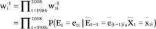
In each period (t), we estimate the probability (wti−1) that the homeownership status was the actual status experienced by the individual (eti), given the history of homeownership (ē(t−1)i) and other confounders, such as income, marital status, and prior wealth (x̅ti).
Multiplying across all years gives the probability that the individual experiences the observed sequence of homeownership outcomes. The IPTW (wi) is the inverse of this probability. Regression models that weight the sample by the IPTWs create a pseudo-population in which homeownership status in each period is independent of prior confounding variables, making it unnecessary to condition on these variables (Robins, Hernán, and Brumback 2000).
Consistent with prior research (Sharkey and Elwert 2011; Wodtke, Harding, and Elwert 2011), we use stabilized IPTWs to reduce the variance of the weights. The stabilized weights can be expressed as
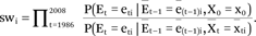
The denominator of the stabilized weight is the inverse of the original weight. The numerator is computed similarly, except that the model conditions on time-invariant baseline traits and prior homeownership status but not other time-varying confounding variables.
Data
The NLSY79 includes 12,686 men and women first interviewed in 1979, when they were ages fourteen to twenty-two. We exclude subsamples discontinued by NLSY79 prior to 2008, including the entire military sample. The remaining 9,763 individuals have subsequently been interviewed annually or biennially (U.S. Bureau of Labor Statistics 2016a), the response rate remaining over 75 percent (U.S. Bureau of Labor Statistics 2016b). Respondents were ages twenty to twenty-eight in the first year asset information was collected (1985) and forty-seven to fifty-six in the most recent year (2012).
Our final models are weighted regressions with years of homeownership between 1986 and 2008 as the main independent variable and midlife wealth, measured as net worth in 2008, as the dependent variable. We describe the wealth data collected by the NLSY79 in more detail later because net worth is one of the time-varying variables in our model of homeownership transitions. In general, net worth in a given survey wave is the sum of respondents’ reported debts and assets of various kinds, including reported home value and mortgage debt. Respondents’ reporting their net worth with error will not bias the estimated wealth benefits of homeownership, provided the error is classical, even if measurement error is greater for some components of net worth than others. However, our results could be biased upward if respondents’ reports of home equity are disproportionately biased upward relative to those of other asset types. This might be true if respondents overestimate the values of their homes, which might be especially likely in the midst of the housing crisis, when home values were falling. However, research suggests that homeowners overestimate the value of their home by only about 6 percent, on average, and homeowners’ errors are not strongly associated with traits of either the owners or the local housing market (Goodman and Ittner 1992). More recent comparisons of data from the Survey of Consumer Finances and the Panel Study of Income Dynamics do not indicate that reported equity in the primary residence is unusually error-prone relative to other components of net worth (Pfeffer et al. 2016).
Our measures of years spent in homeownership assume no homeownership status transitions between waves in which homeownership information is collected; the interwave period is between one and four years. Likewise, to create the estimated probability of a particular homeownership status in an interwave year, we use the most recent available set of covariate values for prediction. Because the stabilized weights include baseline covariates in both the numerator and denominator, the homeownership experiences of the weighted pseudo-population are not independent of these baseline traits, which must also be included in the final outcome model (Wodtke, Harding, and Elwert 2011). We estimate median regressions because they are less sensitive to outliers—a particularly important property given the heavily skewed wealth distribution. Thus, our results estimate the median wealth returns to each year of homeownership. Like ordinary least squares, median regression assumes a constant association between homeownership and wealth across the entire wealth distribution and does not allow us to identify whether the wealth gains of homeownership dispro-portionately accrue to those at the top of the wealth distribution, a point we return to later.
We estimate regression models pooled by race and also separate regression models for Hispanics, non-Hispanic blacks, and non-Hispanic whites, each of which uses IPTWs estimated from race-specific models of homeownership patterns. We do not have a large enough sample size to estimate race-specific models for other racial groups. Our analytic sample for the IPTW models includes 5,636 individuals. Our three race-specific IPTW models include 1,668 blacks, 2,396 whites, and 977 Hispanics.
One limitation of our analysis is that the estimates pertain to a specific birth cohort and period. Home prices fluctuate substantially in real terms and declined precipitously during the Great Recession, as Wolff describes elsewhere in this issue. To test the sensitivity of our results, we use the same model but replace the dependent variable with the respondent’s net worth in 2012, close to the trough of housing values during the Great Recession (Federal Reserve 2016; Dow Jones 2016). We expect lower estimated wealth returns to homeownership in 2012 than in 2008.
Hazard Model Specification
Using discrete-time hazard models and a logit link function, we estimate the risks of entry into first-time homeownership in the next survey year for an individual who has never owned a home (50,180 person-years), entry into a subsequent homeownership spell for a person who has previously owned a home but is not a current homeowner (13,348 person-years), and exit from homeownership for current homeowners (transitions to new homes without intervening spells of non-ownership are not counted) (40,800 person-years). In each wave of the NLSY79, we consider individuals to be homeowners if they report that they or their spouses or partners own or are making payments toward owning their homes. Standard errors are clustered at the individual level in each model. To increase statistical power, our hazard models include all respondents who participated in the current survey wave and provided homeownership data in the next survey wave, even if they do not qualify for our final analytic model because they subsequently attrit. In all models, we use an offset (the log of exposure time) to account for varying durations between homeownership reports due either to the switch from annual to biennial data collection after 1994 or the fact that homeownership was not collected in some post–1985 survey years (1991, 2002, 2006, and 2010). Because of the importance of wealth to our models of selection into homeownership, we use data only from years in which wealth information was collected by the NLSY79.
Although our period of wealth accumulation begins in 1985, we have information on homeownership status since the first wave of the NLSY79 in 1979. Because of the young age of the sample in 1979, we assume that anyone not observed to own a home between 1979 and 1985 has never previously owned a home. Individuals who already owned their homes in 1979 (less than 5 percent of the sample) are left-censored. For these individuals, we assume homeownership began at age eighteen if they were older than eighteen in 1979. If they were eighteen or younger in 1979, we assume they became homeowners in 1979. These assumptions do not affect our calculation of years of homeownership between 1986 and 2008 in our regression models, only the predictors of homeownership transitions used to generate the IPTWs.
The goal of the hazard models is to produce accurate predicted probabilities to use in the IPTWs. To this end, we experimented with model specification, using model fit statistics to adjudicate among alternative specifications of key control variables, such as income. Because of this data-mining process, we do not put great weight on the substantive interpretation of these models, particularly for specific functional forms.1
Age
In each hazard model, age is specified as a linear spline with one knot. The knot is at age thirty-five in the model of first-time transition to homeownership, at age thirty-four in the model of transition to a subsequent spell of homeownership, and at age twenty-seven in the model of exit from homeownership. We also control for birth cohort using the respondent’s age in 1985.
Race
Race is captured with binary variables for whether the respondent is Hispanic, or, if not Hispanic, black, white, Asian American and Pacific Islander, or another race.
Education
We measure educational attainment in the current year in five categories: less than a high school diploma or GED (general educational development test), exactly a high school diploma or GED, some college education, a four-year college degree, or an advanced degree.
Social Origins
Respondents’ social origins are measured with parental education, parental age, whether the respondent was born in the South, and the respondent’s number of siblings, all measured at baseline in 1979. Parental education is measured in the same categories as the respondent’s education and is the maximum among the respondent’s residential parents, if more than one. Parental age is measured as the average between residential parents, if more than one. For respondents not living with any parent at age fourteen, maternal values are used when available. Otherwise, paternal values are used. A dummy variable is set to one if the respondent was born in the American South.
Independent Residence
By definition, homeowners live independently, homeownership being defined by whether the respondent and spouse or partner own or are making payments to own the home. We therefore include a measure of independent residence only in our models of transitions to homeownership. We define the respondent as living independently if in the current survey she is not residing in her parents’ home or in a group home (such as fraternity or sorority house, juvenile detention center, or hospital). In all models, we also include a measure of the number of years since the respondent last lived non-independently.2 Individuals already living independently in 1979 are left-censored. For these individuals, we assume that independent residence began at age eighteen or in 1979, whichever is earliest. In the model of first-time transition to homeownership, years of consecutive independent residence is modeled linearly. In the model of transition to a subsequent spell of homeownership, years of consecutive independent residence enters the model linearly but is top coded at 7. In the model of exit from homeownership, years of consecutive independent residence is modeled as a linear spline with a knot at 2.
Marriage, Gender, and Children
In each wave, we create a binary variable for whether the respondent is currently married. We distinguish between unmarried men and women, incorporating the possibility for a gender gap in homeownership. We recognize that having children may precipitate the decision to buy a home, so we include a dummy variable for whether the respondent has children in the home.
Prior Homeownership Experiences
In the model of repeat homeownership, we include the number of years since the individual was last a homeowner, top coded at 4. For the model of exit from homeownership, we control for the number of years the individual has spent in the current homeownership spell, specified as a linear spline with a knot at 4. To capture unobserved traits possibly associated with enduring risk of homeownership exit, we also include a dummy variable to indicate whether the individual has ever experienced a transition out of homeownership.3
Income
We construct a measure of all income received by the respondent and the respondent’s spouse or partner in the prior calendar year, excluding income of other household members.4 We adjust this measure by the square root of family size (including any cohabiting partner) to more accurately capture disposable income. For the transition to first-time homeownership, we specify income with a linear spline with knots at the 25th and 75th percentiles of the unweighted distribution. For transition to repeat homeownership, we use a linear spline with a knot at the 25th percentile of the unweighted distribution. For transitions out of homeownership, we use a linear spline with knots at the 25th and 50th percentiles of the unweighted distribution.
Wealth
In most years, the NLSY79 has collected information on the respondent’s net worth (1985 through 1990, 1992 through 1994, 1996, 1998, 2000, 2004, 2008, and 2012). Net worth is generally the sum of: housing equity (market value less debt); vehicle equity; cash savings, individual retirement accounts, or stocks and bonds; equity of farms, businesses, or other property owned by the respondent or spouse; and other (residual) valuable items or debts. Beginning in 1988, respondents were also asked to report the value of any rights they hold to estates or trusts. In our models of transitions to homeownership, we log wealth for those with positive net worth and include separate indicators for zero and negative net worth. In the model of transitions out of homeownership, we specify the log of positive net worth as a linear spline with a knot at the 50th percentile of the overall unweighted wealth distribution. We also include indicators for zero and negative wealth. Income and wealth are adjusted to 2012 dollars using the consumer price index. We also top and bottom code positive wealth and income at the 99th and 1st percentiles for each year.
Missing Data and Final Weights
We multiply impute item-missing data on covariates. If homeownership status, which is used to construct the outcome in the hazard models, is missing in any year from 1985 to 2008 in which wealth was also collected, we lack full information on homeownership patterns, so we consider the respondent to have attrited following the last wave in which homeownership information was available and exclude the individual from our IPTW-weighted regressions. We also consider individuals to have attrited if they do not provide information on wealth in 2008—our outcome variable. Following Geoffrey Wodtke, David Harding, and Felix Elwert (2011), we create stabilized weights that account for sample attrition between 1985 and 2008 in the same way as we created stabilized treatment weights, modeling the hazard of attrition at the next wave.
To account for varying probabilities of selection in the initial sample, varying rates of cooperation with the baseline interview, and attrition between 1979 and 1985, we use custom weights supplied by NLSY79 to make the sample of 1985 respondents nationally representative. The product of the stabilized treatment weight, the stabilized attrition weight, and the NLSY79 custom weight (normalized to average one) is the final weight for the individual. Prior to analysis, we also top and bottom code each of the three component weights at the 95th and 5th percentiles of the distribution to reduce the potential for unduly influential outliers.
RESULTS
Table 1 shows descriptive statistics in the sample of individuals and person-year observations used in the IPTW regressions. As expected, race differences in net worth in 2008, at midlife, are vast: an average of $434,000 for whites, versus $247,000 for Hispanics and $126,000 for blacks. Because the distribution of wealth is right-skewed, median values are substantially lower for all groups: $213,000 for whites, $92,000 for Hispanics, and $26,000 for African Americans. Homeownership patterns also differ substantially; whites spend, on average, 14.9 years in homeownership during the twenty-three-year period, versus 10.8 for Hispanics and 7.6 for blacks. Whites are also advantaged with respect to Hispanics and blacks in their social origins; they are less likely to have been born in the South, have fewer siblings, and have parents with higher average education. In terms of achieved characteristics, whites again are most advantaged, having the highest average family incomes, highest probabilities of independent residence, highest marriage rates, and most education.
Descriptive Statistics for the IPTW Sample
The results of the hazard models for transitions into and out of homeownership are provided in table A1. We summarize only the most important findings here. First, prior wealth is strongly positively associated with entrance into both first-time and repeat homeownership and negatively associated with exits from homeownership. These strong associations demonstrate the importance of controlling for prior wealth when considering the association between homeownership patterns and later-life assets. Second, as expected, compared with otherwise similar whites, African Americans and Hispanics are less likely to enter both first and repeat homeownership and are at greater risk of exiting homeownership.
Table 2 presents the results of our regression models. For comparison, we present the results of unweighted regressions as well as our preferred weighted results. We anticipate that weighting will reduce the estimated association between homeownership and subsequent wealth, because the weights remove any association between midlife wealth and homeownership due to the effect of the time-varying variables in our model on both. In the pooled sample, the unadjusted models estimate an additional $9,280 in wealth for every year spent as a homeowner, even after taking into account variation in baseline characteristics, including 1985 wealth. Adjusting for time-varying spurious characteristics, however, reduces the estimated effect by 27 percent, to a benefit of $6,787 per year of homeownership, substantially less than the estimates of Herbert, McCue, and Sanchez-Moyano (2013) and Turner and Luea (2009), which are respectively $9,500 and $13,700. A regression weighted with our attrition weight and the NLSY79 custom weight, but not the treatment weight, increases the estimated association between homeownership and midlife wealth compared to the unweighted model, confirming that the treatment weight is what reduces the estimated association, not the attrition weight or sampling weight.5 Thus, failure to account for dynamic selection into homeownership leads to substantially inflated estimates of the wealth benefits of owning a home.6
Estimated Effects of Homeownership on Wealth
We also find that each additional year of homeownership is associated with an increase of $2,086 in midlife nonhousing wealth, consistent with Di and colleague’s (2007) finding that nonhousing wealth is positively associated with prior homeownership. Thus, although the majority of the wealth benefits of homeownership accrue to housing wealth, the wealth benefits of homeownership do not appear to be limited to home-equity gains.
Our race-specific results show substantial disparities in the wealth returns to homeownership. Whites are estimated to accumulate median wealth gains of $7,602 for every year of homeownership, versus $4,684 for Hispanics and only $3,645 for blacks. Thus the wealth benefits of each year of homeownership are 48 percent as large for blacks as for whites and 62 percent as large for Hispanics. Although adjustments for selection reduce the estimated return to homeownership for each group, the change is proportionally largest for Hispanics. In other words, the differences between Hispanic owners and nonowners, in terms of characteristics conducive to wealth accumulation, are not well captured by baseline covariates alone; differences in circumstances over the observation period also need to be considered. Failure to adjust for the processes by which individuals enter into and maintain homeownership thus not only overstates the wealth benefits of homeownership but also understates the race gap in these benefits; adjusting for dynamic selection processes reduces the Hispanic to white ratio of wealth benefits from homeownership from 86 percent to 62 percent. Our estimate of the relative disadvantage of African Americans’ wealth benefits of homeownership relative to whites’ is also substantially larger than that of Herbert, McCue, and Sanchez-Moyano (2013), who find only a 20 percent gap.
As expected, the estimated wealth returns to homeownership are lower when wealth is measured in 2012. In the pooled sample, each additional year of homeownership is associated with an increase in midlife wealth of $4,424 in 2012, 35 percent less than when the outcome is 2008 wealth. This decline is not primarily due to declines in the relative value of homeownership but to declines in overall wealth levels, compressing absolute gains; when we replicate the models using the log of net worth as the outcome, restricting the sample to those with positive net worth, we see that, on average, the proportional benefits of homeownership for wealth declined only modestly between 2008 and 2012, from about 4.9 percent to about 4.7 percent.
Given that Hispanics and African Americans were hit particularly hard by the Great Recession in terms of proportional declines in wealth and home equity (Grinstein-Weiss, Key, and Carrillo 2015; McKernan et al. 2013), we might expect that variation by race in the wealth returns to homeownership would be even larger in 2012 than in 2008. However, we find similar disparities in 2012 as 2008. In 2012, the wealth benefits of each year of homeownership are 50 percent as large for blacks and 62 percent as large for Hispanics as for whites.
One natural question is whether the absolute wealth benefits of homeownership are lower for racial minorities simply because overall wealth levels are lower.7 Furthermore, our estimates of the median wealth benefits of homeownership may mask greater absolute returns to homeownership for high-wealth individuals. To investigate this possibility, we repeat our models using the log of net worth among those with positive net worth as the outcome rather than raw wealth values. In proportional terms, among those with positive net worth, whites have the lowest wealth returns to homeownership in both 2008 and 2012. It is tempting to interpret these results as estimating the returns for every $1 invested in home purchase, but this is not the case: the models predict 2008 (or 2012) wealth with years of homeownership, not the return on dollars invested in housing. The absolute models assume that an extra year of homeownership has a constant effect on midlife wealth across the wealth distribution, whereas the proportional models assume that it benefits individuals by a constant proportion across the wealth distribution. Given that wealth levels are substantially lower for racial minorities than whites, regardless of homeowner status, similar proportional gains from homeownership will translate into larger absolute gains for whites; this is a purely mechanical relationship and does not by itself reveal anything about the social process underlying racial variation in the wealth benefits of homeownership.8
A more challenging question is whether equality in the wealth benefits of homeownership should be interpreted as a statement about absolute or proportional equality. If the goal is to assess whether the housing market is biased against minority homeowners, proportional equality might be the preferred standard. However, even if the wealth returns to homeownership are proportional to wealth and homogeneous by race, it tells us only that the pervasive wealth disadvantage that racial minorities experience relative to whites in both housing and nonhousing wealth limits minority homeowners’ abilities to keep pace with the absolute wealth accumulation rates of their white peers. Beyond standard income and investment considerations, recent research highlights that African American families’ wealth positions are disadvantaged by negative health shocks (Thompson and Conley, this volume) and incarceration (Schneider and Turney 2015; Sykes and Maroto, this volume).
To explore the role of homeownership in racial wealth gaps, we decompose how closing the race gap in homeownership rates would change the race gap in the total wealth benefits of homeownership, versus the effect of eliminating the gap in the returns to each year of homeownership. As shown in table 3, we begin by simulating the wealth gains from homeownership for whites, blacks, and Hispanics who experienced the race-specific median years of homeownership and race-specific median returns to each year of homeownership between 1986 and 2008. Disparities are large; in this simulation, whites accumulate a total of $129,000 for homeownership, versus $52,000 for Hispanics and $18,000 for blacks. In other words, the gains are only 40 percent as large for Hispanics and only 14 percent as large for blacks. Now we simulate the total midlife wealth gains from homeownership under the counterfactual scenario that each group owns a home for seventeen years during the period—the median for whites—but experiences race-specific wealth benefits for each year of homeownership. The gaps in accumulated wealth due to homeownership decrease for both groups; the cumulative gains for Hispanics are now 62 percent and for blacks 48 percent as large as for whites. When we alternatively hold constant the wealth returns to a year of homeownership at the estimated level for whites ($7,602) but allow each race to have different exposure to homeownership, Hispanics accumulate 65 percent and blacks 29 percent as much as whites. Thus, for both blacks and Hispanics, race disparities in rates of homeownership and returns to homeownership are both substantial contributors to the race gap in wealth accumulated from homeownership. For Hispanics, the two factors contribute approximately equally, and, for blacks, the role of differences in rates of homeownership is larger.
Simulated Total Wealth Benefits of Homeownership
The three rightmost columns of table 3 simulate the role of homeownership in the race gap in midlife wealth. We simulate median midlife wealth levels by race in the absence of homeownership by subtracting from observed median wealth levels the simulated total wealth benefits of homeownership given race-specific homeownership rates and returns to homeownership, as calculated in the left-hand columns. To these baseline levels, we then add wealth gains from homeownership in three alternative scenarios: years of homeownership equalized at the white median; returns to years of homeownership equalized at the white median; and total wealth benefits of homeownership equalized setting both years of homeownership and the returns to years of homeownership to the white median for all respondents. At midlife, the observed median wealth of Hispanics and African Americans is 43 percent and 12 percent that of whites, respectively. In the counterfactual simulation of no homeownership, the analogous numbers are 48 percent and 9 percent, respectively. Although whites are advantaged in wealth in part because of their higher rates of homeownership and greater wealth returns per year of homeownership, these gains are similar to whites’ advantage in other wealth-generating processes; disparities in homeownership experiences contribute to the race gap in wealth, but not uniquely so.
Equalizing homeownership rates and the wealth benefits per year of homeownership, however, could substantially narrow race gaps in wealth. Under this simulated scenario, Hispanic median midlife wealth is 80 percent and African American 64 percent that of whites. Although substantial race gaps in midlife wealth remain even in this optimistic scenario, the results show that equality in wealth benefits of homeownership could substantially narrow them.
Our analyses are, of course, imperfect. Although our models are designed to account for dynamic selection into homeownership, they have the same limitations as all observational studies and depend on the assumption that we have captured wealth-relevant differences between homeowners and renters with our control variables. Although prior research does not suggest substantial bias due to reporting error, overestimates of home values relative to other assets could upwardly bias the homeownership wealth returns. Our results suggest that prior estimates have overstated the wealth benefits of homeownership, and the true effect could be even lower than our results suggest.
Our results also apply to the experiences of a particular cohort at a particular point in their lives and in a particular macroeconomic context. Although we find substantial wealth benefits from homeownership regardless of whether wealth is measured in 2008 or 2012, cohorts of homeowners entering the housing market after the Great Recession may have different experiences. The observed variation in the wealth benefits of homeownership by race may also be context-specific and sensitive to the overall wealth gap between whites, African Americans, and Hispanics. For example, the Hispanics included in our sample were all observed in the United States in 1979, when they were young adults, so the estimates may not reflect the benefits of homeownership for recent Hispanic immigrants.
Finally, the simulations in table 3 are descriptive rather than causal. They illustrate how race gaps in wealth would change under various illustrative counterfactual scenarios, but they are not designed to incorporate, for example, the possibility that changes in homeownership rates would also change the returns to homeownership.
CONCLUSIONS
Home equity is the largest component of most American asset portfolios, and homeownership is widely assumed to be a pathway to wealth accumulation. Yet prior estimates of the long-term benefits of homeownership for later-life wealth have typically ignored the possibility of spurious events during the observation window that affect both transitions into and out of homeownership and subsequent wealth. Our results confirm that homeownership has substantial wealth benefits. Each additional year spent as a homeowner is associated with about $6,800 more in midlife wealth in 2008. Comparing our weighted and unweighted results, we find that accounting for the dynamic relationships between wealth, homeownership, and other wealth-enhancing characteristics reduces the wealth benefits of homeownership by 27 percent. In 2012, each year of homeownership between 1986 and 2008 is associated with about $4,400 more in midlife wealth. Thus, even in the midst of the housing crisis, time spent in homeownership positively affected wealth. However, our estimates of the wealth benefits of homeownership are smaller than previous estimates (Herbert, McCue, and Sanchez-Moyano 2013; Turner and Luea 2009).
Although housing markets do not appear to uniquely disadvantage African Americans and Hispanics—eliminating homeownership would not substantially change the race gap in wealth—altering their homeownership experiences to be comparable to those of whites would substantially narrow race gaps in midlife wealth. We find that, compared with whites, blacks and Hispanics are disadvantaged in three distinct ways. First, as shown in our descriptive results, they have, on average, characteristics that are less likely to facilitate entering and maintaining homeownership. As a result, they participate less in this wealth-generating state. Programs and policies designed to reduce racial disparities in other domains, including education and income, may thus have spillover effects on the race gap in homeownership and wealth.
Second, even holding other determinants of homeownership constant, blacks and Hispanics have lower rates of entry into homeownership and higher rates of exit than whites, further depressing their accumulated years of homeownership. Stricter enforcement of antidiscrimination laws in housing markets might help close the race gap in access to homeownership, particularly given evidence that blacks face higher rates of rejection for mortgage applications than comparable whites (Charles and Hurst 2002). Recent analyses have also implicated residential segregation in the concentration of subprime lending among black and Hispanic homeowners (Hwang, Hankinson, and Brown 2015). It is possible that stricter regulations in subprime lending would reduce race disparities in risk of homeownership exit.
Third, for every year they spend as homeowners, blacks and Hispanics receive lower median wealth returns than whites do. Disparities in homeownership rates and in the returns to homeownership both contribute substantially to the gaps by race in long-term wealth accumulation from homeownership. One possible mechanism for equalizing returns is to invest in predominantly black and Hispanic neighborhoods, given that other scholars have attributed lower rates of home appreciation for black homeowners in part to racial segregation (Flippen 2004; Oliver and Shapiro 2006). However, the results from our models of log wealth demonstrate that minority homeowners do not experience lower proportional wealth returns to homeownership, but the substantially lower average wealth positions of nonwhite owners and nonowners alike imply that these proportional returns translate into far smaller absolute wealth benefits. Policies aimed only at housing markets, therefore, may have limited effect on equalizing the wealth returns to years of homeownership without also addressing other sources of the residual race gap in wealth above and beyond race differences in income. Future research is needed to further investigate the sources of this residual gap and identify policy levers to narrow it.
Acknowledgments
This research was supported in part by an Emerging Scholars Small Grant from the University of Wisconsin Institute for Research on Poverty. An earlier version of this paper was presented at the 2015 annual meeting of the Population Association of America. We are grateful to Fangsheng Zhu for research assistance and to Vanesa Estrada-Correa, Fabian Pfeffer, Bob Schoeni, and anonymous reviewers for helpful comments.
Appendix
Discrete-Time Hazard Models of Entry to and Exit from Homeownership
FOOTNOTES
↵1. The hazard models used to create the numerator of the stabilized inverse probability of treatment weights and the attrition weights use only time-invariant covariates set to their baseline values in 1985. For these models we rely on linear specifications of the baseline covariates.
↵2. We assume stability in independent residence between reports for up to two years following a report.
↵3. We assume stability in homeownership status between reports, for up to three years following a report.
↵4. Our measure of income includes inheritance and gifts from relatives received in the last calendar year. It is possible that transfers are endogenous with intended home purchase. Estimates of the effect of homeownership on midlife wealth were nearly identical when inheritance and gifts were excluded from the income measure.
↵5. In a supplemental model, we replaced the product of our attrition weight and NLSY79 custom weight for 1985 respondents with a single NLSY79 custom weight designed to make the sample of respondents observed in every wave between 1985 and 2008 (inclusive) in which wealth data were collected nationally representative. In other words, we used the NLSY79’s combined sampling and attrition weight rather than our own. The results were similar: an estimated gain of $6,311 in midlife wealth per year of homeownership, versus $6,787 in the main model.
↵6. Furthermore, without adjustments for dynamic selection, controls for wealth at baseline have a relatively small effect on the estimated wealth benefits of homeownership. In a supplemental unweighted model that further omitted wealth in 1985 from the baseline model, the estimated wealth benefit for each year of homeownership was $9,783. Adjusting for wealth at baseline therefore reduces this naïve estimate by only 5 percent, versus 31 percent relative to the naïve model when we implement our preferred adjustment for dynamic selection.
↵7. Similarly, we find that the absolute wealth returns to homeownership were lower for less-educated than more-educated whites (the sample is not large enough to do a similar analysis for Hispanics and African Americans).
↵8. Restricting the log of net worth models to respondents with positive net worth omits 15 and 18 percent of respondents in 2008 and 2012, respectively. If this selection process varies by race, differences in the sample could contribute to the white advantage in absolute but not proportional wealth returns to homeownership. We do not find support for this possibility in 2008: absolute wealth returns estimated on a sample of respondents with positive net wealth show wealth returns to homeownership about twice as large for whites as for either Hispanics or African Americans. However, in 2012, when the sample is restricted to respondents with positive net worth, we find that Hispanics have absolute wealth returns to homeownership similar to those of whites, and the black-white gap in the returns to homeownership is somewhat diminished. Therefore, in 2012 race differences in selection into positive net worth may contribute to the lower proportional returns to homeownership for whites.
- Copyright © 2016 by Russell Sage Foundation. All rights reserved. Printed in the United States of America. No part of this publication may be reproduced, stored in a retrieval system, or transmitted in any form or by any means, electronic, mechanical, photocopying, recording, or otherwise, without the prior written permission of the publisher. Reproduction by the United States Government in whole or in part is permitted for any purpose. This research was supported in part by an Emerging Scholars Small Grant from the University of Wisconsin Institute for Research on Poverty. An earlier version of this paper was presented at the 2015 annual meeting of the Population Association of America. We are grateful to Fangsheng Zhu for research assistance and to Vanesa Estrada-Correa, Fabian Pfeffer, Bob Schoeni, and anonymous reviewers for helpful comments. Direct correspondence to: Alexandra Killewald at killewald{at}fas.harvard.edu, 436 William James Hall, Harvard University, 33 Kirkland St., Cambridge, MA 02138; and Brielle Bryan at briellebryan{at}g.harvard.edu, 432 William James Hall, Harvard University, 33 Kirkland St., Cambridge, MA 02138.
Open Access Policy: RSF: The Russell Sage Foundation Journal of the Social Sciences is an open access journal. This article is published under a Creative Commons Attribution-NonCommercial-NoDerivs 3.0 Unported License.
REFERENCES
In this issue


Jump to section
Related Articles
Cited By...
- No citing articles found.